The open() function opens a file. It takes two parameters: a filename plus an optional mode string, which can contain one or more of these characters:
'r' – open for
reading (default)
'w' – open for
writing. If the file already exists, its existing contents will be
lost!
'a' – append
to an existing file, or create a new file if the file does not exist
already
't' – text
mode (default)
'b' – binary
mode
If you don't specify a mode string, the file will be opened for reading in text mode.
When you open a file in text mode, Python will perform universal newline translation, i.e. translate any sort of newlines to '\n'. We will only use text mode in this course.
open() returns a file object. When reading,
the file object is iterable: you can loop over it with for
to receive a sequence of lines, just like with sys.stdin. When a file
is opened for writing, you may
write lines to the file by calling the write() method on the file
object once for each output line.
When we are finished reading or writing data, you should call close() to close the file.
Here's a program that opens two files called 'input.txt' and 'output.txt'. It reads lines from the input file and writes them to the output file, duplicating every line as it writes:
input = open('input.txt', 'r')    # open for reading ('r' is default mode)
output = open('output.txt', 'w')     # open for writing

for line in input:
    output.write(line)      # write line to output
    output.write(line)      # write it again

input.close()
output.close()
You can read about more methods for input and output in our Python quick library reference.
with statementWhenever
you open a file, you'll want to close it, even if your program exits
unexpectedly with an error. Python has a special statement that makes
this easy. The with
statement assigns a file
object (or other resource) to a variable, then runs a block of code.
When the block of code exits for any reason, the object is
automatically closed, just as if you had called close() on the
object.
Let's
rewrite the previous program using 'with':
with open('input.txt', 'r') as input:    # open for reading ('r' is default mode)
    with open('output.txt', 'w') as output:     # open for writing
        for line in input:
            output.write(line)      # write line to output
            output.write(line)      # write it again
It's good practice to use 'with' whenever you open a file, to ensure that the file will be closed even if the program exits with an error.
In fact with
also works with other types of objects that need to be closed, such
as network sockets. We may see some of these later in this course.
When we run a program from the command line, we may specify command-line arguments. For example:
$ python prog.py hello one two three
In a Python program, sys.argv holds a list of all command-line arguments. Actually the first element in the list is the name of the program itself, and subsequent elements hold the arguments. For example, suppose that prog.py holds this program:
import sys

print(sys.argv)
Let's run it:
$ python3 prog.py hello one two three
['prog.py', 'hello', 'one', 'two', 'three']
As an example, let's write a program that imitates the Unix utility 'wc' ("word count"), which prints out the number of lines, words, and characters in a file:
import sys

if len(sys.argv) != 2:
    print(f'usage: {sys.argv[0]} <filename>')
    exit()

filename = sys.argv[1]
chars = words = lines = 0

with open(filename) as f:
    for line in f:
        chars += len(line)
        words += len(line.split())
        lines += 1

print(f'{lines} lines, {words} words, {chars} chars')
Notice that the program prints out a usage message if we attempt to invoke it without arguments. This is a good practice:
$ python wc.py
usage: wc.py <filename>
Let's use the program to count the lines, words and characters in its own source code:
$ python wc.py wc.py
16 lines, 43 words, 324 chars
This matches the counts printed by the Unix wc utility itself:
$ wc wc.py
 16  43 324 wc.py
Command-line programs will often accept arguments with names beginning with a hyphen, such as -d or ‑e. Typically these denote options that affect a program's behavior.
As another example, let's implement a simple variant of the Unix utility 'grep', which searches for a string in a given file, and prints out all lines containing the string. Our program will accept two options:
-i: search
case-insensitively, i.e. "horse" will match "HoRsE"
-v: invert
matches, i.e. print out lines that do not contain the given
string
Here's the program:
import sys

def usage():
    print(f'usage: {sys.argv[0]} [-i] [-v] <string> <filename>')
    exit()

insensitive = invert = False

i = 1
while i < len(sys.argv):
    arg = sys.argv[i]
    if arg.startswith('-'):
        if arg == '-i':
            insensitive = True
        elif arg == '-v':
            invert = True
        else:
            usage()
    else:
        break    # end of options
    i += 1

if len(sys.argv) - i < 2:
    usage()

find = sys.argv[i]
if insensitive:
    find = find.lower()
filename = sys.argv[i + 1]

with open(filename) as f:
    for line in f:
        line = line.rstrip()
        if insensitive:
            line = line.lower()
        match = find in line
        if (match and not invert) or (not match and invert):
            print(line)
Let's use it to find all lines containing "sys" in the program's own source code:
$ python grep.py -i sys grep.py
import sys
    print(f'usage: {sys.argv[0]} [-i] [-v] <string> <filename>')
while i < len(sys.argv):
    arg = sys.argv[i]
if len(sys.argv) - i < 2:
find = sys.argv[i]
filename = sys.argv[i + 1]In Python, you may use if
and else inside an expression;
this is called a conditional expression.
For example, consider this code:
if x > 100:
    print('x is big')
else:
    print('x is not so big')
We may rewrite it using a conditional expression:
print('x is ' + ('big' if x > 100 else 'not so big'))As another example, here is a function that takes two integers and returns whichever has the greater magnitude (i.e. absolute value):
def greater(i, j):
   if abs(i) >= abs(j):
       return i
   else:
       return j
We can rewrite it using a conditional expression:
def greater(i, j):
    return i if abs(i) >= abs(j) else j
A conditional expression always has the form
expression
if
condition else
expression
The
keyword else must
always be present (unlike in an ordinary if
statement).
(If you already know C or another C-like language, you may notice this feature's resemblance to the ternary operator (? :) in those languages.)
A tuple in Python is an immutable sequence. Its length is fixed, and you cannot update values in a tuple. Tuples are written with parentheses:
>>> t = (3, 4, 5)
>>> t[0]
3
>>> t[2]
5
Essentially a tuple is an immutable list. All sequence operations will work with tuples: for example, you can access elements using slice syntax, and you can iterate over a tuple:
>>> t = (3, 4, 5, 6)
>>> t[1:3]
(4, 5)
>>> for x in t:
...    print(x)
...
3
4
5
6
>>>
The built-in function tuple() will convert any sequence to a tuple:
>>> tuple([2, 4, 6, 8])
(2, 4, 6, 8)

>>> tuple(range(10))
(0, 1, 2, 3, 4, 5, 6, 7, 8, 9)
We will often use tuples in our code. They are (slightly) more efficient than lists, and their immutability makes a program easy to understand, since when reading the code you don't need to worry about if/when their elements might change.
A tuple of two elements is called a pair. A tuple of three elements is called a triple. Usually in our code we will use tuples when we want to group a few elements together. For example, a pair such as (3, 4) is a natural way to represent a point in a 2-dimensional space. Similarly, a triple such as (5, 6, -10) may represent a point in 3-space.
In Python we may assign to multiple variables at once to unpack a list or tuple:
>>> [a, b, c] = [1, 3, 5]
>>> a
1
>>> b
3
>>> c
5

>>> (x, y) = (4, 5)
>>> x
4
>>> y
5
In these assignments you may even write a list of variables on the left, without list or tuple notation:
>>> a, b, c = [1, 3, 5]
>>> x, y = (4, 5)
On the right side, you may write a sequence of values without brackets or parentheses, and Python will automatically form a tuple:
>>> t = 3, 4, 5
>>> t
(3, 4, 5)
In fact Python will freely convert between sequence types in assignments of this type. For example, all of the following are valid:
>>> a, b, c = 3, 4, 5
>>> [d, e] = (10, 11)
>>> f, g, h = range(3)   # sets f = 0, g = 1, h = 2
These "casual" conversions are often convenient. (They would not be allowed in stricter languages such as Haskell.)
Finally, note that variables on the left side of such as assignment may also appear on the right. The assignment is simultaneous: the new values of all variables on the left are computed using the old values of variables on the right. For example, we may swap the values of two variables like this:
>>> x, y = 10, 20
>>> x
10
>>> y
20
>>> x, y = y, x
>>> x
20
>>> y
10
In fact we already used this form of multiple simultaneous assignment when we implemented Euclid's algorithm in our algorithms class a couple of weeks ago. Here is that code again:
# compute gcd(a, b)
while b != 0:
a, b = b, a % bA list of tuples is a convenient representation for a set of points. Let's write a program that will read a set of points from standard input, and determine which two points are furthest from each other. The input will contain one point per line, like this:
2 5
6 -1
-3 6
...
Here is the program:
import math
import sys

points = []
for line in sys.stdin:
    xs, ys = line.split()    # multiple assignment
    point = (int(xs), int(ys))
    points.append(point)

print(points)

m = 0   # maximum so far

for px, py in points:
    for qx, qy in points:
        dist = math.sqrt((px - qx) ** 2 + (py - qy) ** 2)
        if dist > m:
            m = dist

print(m)
The line xs, ys = line.split() is a
multiple assignment as we saw in the previous section. Note that this
will work only if each input line contains exactly two words. If
there are more or fewer, it will fail:
>>> xs, ys = '20 30'.split()   # OK

>>> xs, ys = '20 30 40'.split()
Traceback (most recent call last):
  File "<stdin>", line 1, in <module>
ValueError: too many values to unpack (expected 2)
Above, notice that a for loop may assign to multiple variables on each iteration of the loop when iterating over a sequence of sequences (as in this example). We could instead write
for p in points:
    for q in points:
        px, py = p
        qx, qy = q
but the form "for px, py in points"
is more convenient.
The program above is a bit inefficient, since it will compute the distance between each pair of points twice. We may modify it so that the distance between each pair is computed only once, like this:
n = len(points)
for i in range(n):
    for j in range(i + 1, n):
        px, py = points[i]
        qx, qy = points[j]
        dist = math.sqrt((px - qx) ** 2 + (py - qy) ** 2)
        if dist > m:
            m = dist
The first time the inner loop runs, it will iterate over (N - 1) points. The second time it runs, it will iterate over (N - 2) points, and so on. The total running time will be O((N - 1) + (N - 2) + ... + 1) = O(N²). So it's still quadratic, though about twice as efficient as the previous version.
Could we make the program more efficient? In fact an algorithm is known that will find the two furthest points in O(N log N). You might learn about this algorithm in a more advanced course about computational geometry.
A recursive function calls itself. Recursion is a powerful technique that can help us solve many problems.
When we solve a problem recursively, we express its solution in terms of smaller instances of the same problem. The idea of recursion is fundamental in mathematics as well as in computer science.
As a first example, suppose we we'd like to write a function that computes n! for any positive integer n. Recall that
n! = n · (n – 1) · … · 3 · 2 · 1
We may write this function iteratively, i.e. using a loop:
def factorial_iter(n):
    p = 1

    for i in range(1, n + 1):
        p *= i

    return p
Alternatively, we can rewrite this function using recursion. Now it calls itself:
def factorial(n):
    if n == 0:
        return 1     # 0! is 1

    return n * factorial(n - 1)
Whenever we write a recursive function, there is a base case and a recursive case.
The base case is an instance that we can solve immediately. In the function above, the base case is when n == 0. A recursive function must always have a base case – otherwise it would loop forever since it would always call itself!
In the recursive case, a function calls itself, passing it a smaller instance of the given problem. Then it uses the return value from the recursive call to construct a value that it itself can return.
In the recursive case in this example, we
recursively call factorial(n -
1). We then multiply its return value by n, and
return that value. That works because
n! = n · (n – 1)! whenever n ≥ 1
(In fact, we may treat this equation as a recursive definition of the factorial function, mathematically speaking.)
How does this function work, exactly? Suppose that we call factorial(3). It will call factorial(2), which calls factorial(1), which calls factorial(0). The call stack in memory now looks like this:
factorial(3)
→ factorial(2)
  → factorial(1)
    → factorial(0)
Now
factorial(0) returns 1 to its caller factorial(1).
factorial(1) takes this value 1, multiplies it by n = 1 and returns 1 to factorial(2).
factorial(2) takes this value 1, multiplies it by n = 2 and returns 2 to factorial(3).
factorial(3) takes this value 2, multiplies it by n = 3 and returns 6.
We see that given any n, the function returns the sum 1 * 2 * 3 * … * n = n!.
We have seen that we can write the factorial function either iteratively (i.e. using loops) or recursively. In theory, any function can be written either iteratively or recursively. We will see that for some problems a recursive solution is easy and an iterative solution would be quite difficult. Conversely, some problems are easier to solve iteratively. Python lets us write functions either way.
Here is some general advice for writing a recursive function. First look for a base case where the function can return immediately. (In some problems there will actually be more than one base case.) Now you need to write the recursive case, where the function calls itself. At this point you may wish to pretend that the function "already works". Write the recursive call and believe that it will return a correct solution to a subproblem, i.e. a smaller instance of the problem. Now you must somehow transform that subproblem solution into a solution to the entire problem, and return it. This is really the key step: understanding the recursive structure of the problem, i.e. how a solution can be derived from a subproblem solution.
Here's another example. Consider this implementation of Euclid's algorithm that we saw in Introduction to Algorithms:
# gcd, iteratively
def gcd(a, b):
    while b > 0:
        a, b = b, a % b

    return a
We can rewrite this function using recursion:
# gcd, recursively
def gcd(a, b):
    if b == 0:
        return a

    return gcd(b, a % b)
Broadly speaking, we will see that "easy" recursive
functions such as gcd call themselves
only once, and it would be straightforward to write them either
iteratively or recursively. Soon
(in our algorithms class) we will see recursive functions that
call themselves two or more times. Those functions will let us solve
more difficult tasks that we could not easily solve iteratively.
Here is another example of a recursive function:
def hi(x):
    if x == 0:
        print('hi')
        return

    print('start', x)
    hi(x - 1)
    print('done', x)
If we call hi(3), the output will be
start 3
start 2
start 1
hi
done 1
done 2
done 3
Be sure you understand why the lines beginning with 'done' are printed. hi(3) calls hi(2), which calls hi(1), which calls hi(0). At the moment that hi(0) runs, all of these function invocations are active and are present in memory on the call stack:
hi(3)
→ hi(2)
  → hi(1)
    → hi(0)
Each function invocation has its own value of the parameter x. (If this procedure had local variables, each invocation would have a separate set of variable values as well.)
When hi(0) returns, it does not exit from this entire set of calls. It returns to its caller, i.e. hi(1). hi(1) now resumes execution and writes 'done 1'. Then it returns to hi(2), which writes 'done 2', and so on.
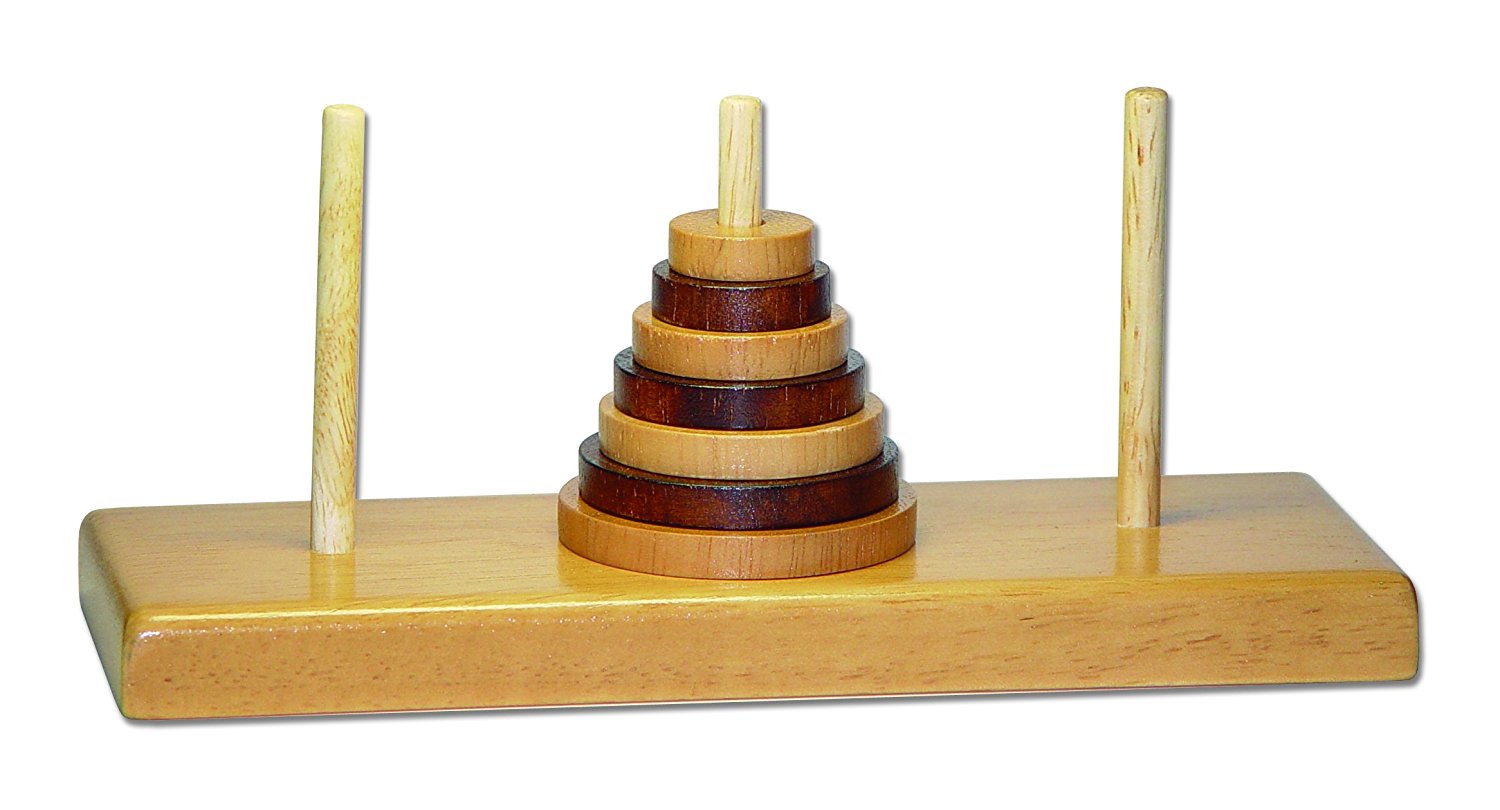
The Tower of Hanoi is a well-known puzzle that looks like this:
The puzzle has 3 pegs and a number of disks of various sizes. The player may move disks from peg to peg, but a larger disk may never rest atop a smaller one. Traditionally all disks begin on the leftmost peg, and the goal is to move them to the rightmost.
Supposedly in a temple in the city of Hanoi there is a real-life version of this puzzle with 3 rods and 64 golden disks. The monks there move one disk each second from one rod to another. When they finally succeed in moving all the disks to their destination, the world will end.
The world has not yet ended, so we can write a program that solves a version of this puzzle with a smaller number of disks. We want our program to print output like this:
move disk 1 from 1 to 2
move disk 2 from 1 to 3
move disk 1 from 2 to 3
move disk 3 from 1 to 2
…
To solve this puzzle, the key insight is that a simple recursive algorithm will do the trick. To move a tower of disks 1 through N from peg A to peg B, we can do the following:
Move the tower of disks 1 through N-1 from A to C.
Move disk N from A to B.
Move the tower of disks 1 through N-1 from C to B.
The program below implements this algorithm:
# move tower of n disks from fromPeg to toPeg
def hanoi(n, fromPeg = 1, toPeg = 3):
  if n == 0:
    return
  other = 6 - fromPeg - toPeg
  hanoi(n - 1, fromPeg, other)
  print(f'move disk {n} from {fromPeg} to {toPeg}')
  hanoi(n - 1, other, toPeg)
We can compute the exact number of moves required to solve the puzzle using the algorithm above. If M(n) is the number of moves to move a tower of height n, then we have the recurrence
M(n) = 2 ⋅ M(n–1) + 1
The solution to this recurrence is, exactly,
M(n) = 2n – 1
Similarly, the running time of our program above follows the recurrence
T(n) = 2 ⋅ T(n–1) + O(1)
And the program runs in time T(n) = O(2n).
It will take 264 - 1 seconds for the monks in Hanoi to move the golden disks to their destination tower. That is far more than the number of seconds that our universe has existed so far.