
Last week we learned about binary search trees, and discussed how to add an element to a binary search tree or check whether an element is already present.
Deleting a value from a binary search tree is a bit trickier. It's not hard to find the node to delete: we just walk down the tree, just like when searching or inserting. Once we've found the node N we want to delete, there are several cases.
If N is a leaf (it has no children), we can just remove it from the tree.
If N has only a single child, we replace N with its child. For example, we can delete node 15 in the binary tree above by replacing it with 18. To accomplish this, we'll change node 20's left pointer to point to node 18 instead of node 15.
If N has two children, then we will replace its value by the next largest value in the tree. To do this, we start at N's right child and follow left child pointers for as long as we can. This wil take us to the smallest node in N's right subtree, which must be the next largest node in the tree after N. Call this node M. We can easily remove M from the right subtree: M has no left child, so we can remove it following either case (a) or (b) above. Now we set N's value to the value that M had.
As a concrete example, suppose that we want to delete the root node (with value 10) in the tree above. This node has two children. We start at its right child (20) and follow its left child pointer to 15. That’s as far as we can go in following left child pointers, since 15 has no left child. So now we remove 15 (following case b above), and then replace 10 with 15 at the root.
(Alternatively, we could delete node N by replacing its value with the next smallest value in the tree. That approach is symmetric and would work equally well. To find the next smallest value, we can start at N's left child and follow right child pointers for as long as we can.)
We won't give an implementation of this operation here, but writing this yourself is an excellent (and somewhat challenging) exercise.
It is not difficult to see that the add,
remove and contains operations described
above will all run in time O(h), where h is the height of a binary
search tree. What is their running time as a function of N, the
number of nodes in the tree?
First consider a complete binary search tree. As
we saw above, if a complete tree has N nodes then its height is
h = log2(N + 1) – 1 ≈ log2(N)
– 1 = O(log N). So add, remove, and
contains will all run in time O(log N).
Even if a tree is not complete, these operations will run in O(log N) time if the tree is not too tall given its number of nodes N, specfically if its height is O(log N). We call such a tree balanced.
Unfortunately not all binary trees are balanced. Suppose that we insert values into a binary search tree in ascending order:
t = TreeSet()
for i in range(1, 1000):
    t.add(i)
The tree will look like this:

This tree is completely unbalanced. It basically
looks like a linked list with an extra None
pointer at every node. add, remove and
contains will all run in O(N) on this tree.
How can we avoid an unbalanced tree such as this one? There are two possible ways. First, if we insert values into a binary search tree in a random order then that the tree will almost certainly be balanced. We will not prove this fact here (you might see a proof in the Algorithms and Data Structures class next semester).
Unfortunately it is not always practical to insert in a random order – for example, we may be reading a stream of values from a network and may need to insert each value as we receive it. So alternatively we can use a more advanced data structure known as a self-balancing binary tree, which automatically balances itself as values are inserted. Two examples of such structures are red‑black trees and AVL trees. We will not study these in this course, but you will see them in Algorithms and Data Structures next semester. For now, you should just be aware that they exist. In a self-balancing tree, the add(), remove() and contains() methods are all guaranteed to run in O(log N) time, for any possible sequence of tree operations.
We have already seen several abstract data types: stacks, queues, and sets. Another abstract data type is a dictionary (also called a map or associative array), which maps keys to values. It provides these operations:
A dictionary cannot contain the same key twice. In other words, a dictionary associates a key with exactly one value.
This type should be familiar, since we have used Python's dictionaries, which are an implementation of this abstract type.
In general, given any implementation of the set abstract data type, it is usually easy to modify it to implement a dictionary.
For example, we can use a binary search tree to implement a dictionary. To do so, we only need to make a small change to the binary search tree code we saw last week: now each node will store a key-value pair. In Python, our Node class will look like this:
class Node:
    def __init__(self, key, val, left, right):
        self.key = key
        self.val = val
        self.left = left
        self.right = right
The lookup() operation will be similar to the set operation contains(): it will search the tree for a node with the given key; if found, it will return the corresponding value. The dictionary operations set() and remove_key() will also be similar to the set operations add() and remove(). I won't implement these operations here; if you like, you can write them yourself as an easy exercise.
Let's consider another abstract data type, namely a dynamic array. A dynamic array d has these operations:
This interface probably looks familiar, since a Python list is a dynamic array!
In lower-level languages such as C an array typically has a fixed size. Let's now implement a dynamic array in Python, using only fixed-size arrays. That means that in our implementation we can allocate an array using an expression such as '10 * [None]', but we may not call the append() method to expand an existing array.
We'll use a class with two attributes: a
fixed-size array a plus an attribute n that
indicates how many elements in the array are currently in use. Each
time we add an element to the dynamic array, we first check if the
underlying array a is full. If so, we'll allocate a new
array that is 10 elements larger, and copy all elements from the old
array to the new array.
Here is our implementation:
class DynArray:
    def __init__(self):
        self.a = 10 * [None]
        self.count = 0

    def get(self, i):
        return self.a[i]

    def set(self, i, x):
        self.a[i] = x

    def length(self):
        return self.count

    def add(self, x):
        if self.count == len(self.a):       # array self.a is full
            self.a = self.a + 10 * [None]   # expand array
        self.a[self.count] = x
        self.count += 1
Note that the line with the comment "expand array" above does not grow the original array self.a in place. The + operator allocates a new array, so it is equivalent to this code:
b = (self.count + 10) * [None]   # allocate an array with 10 extra elements
for i in range(self.count):
    b[i] = self.a[i]
self.a = b
Our class works:
>>> d = DynArray()
>>> for x in range(1, 1001):
...   d.add(x)
...
>>> d.get(100)
101
>>> d.get(500)
501
Now suppose that we create a DynArray and add N elements in a loop:
d = DynArray()
for i in range(N):
    d.add(i)
How long will this take, as a big-O function of N?
The total time will be the time for all the resize operations, plus the extra work done by the last two lines in the add() method. The extra work takes O(1) per element added, so the total time of the extra work is O(N).
A single resize operation from size S to size S + 10 must allocate an array of size S + 10, then copy S elements to the new array. Both of these operations take time O(S), so the total time for a single resize operation from size S is O(S). Then the total time for all the resize operations will be
O(10 + 20 + 30 + … + N) = O(1 + 2 + 3 + … + (N / 10)) = O((N / 10)2) = O(N2).
So the total time for the loop to run will be O(N) + O(N2) = O(N2). And so the average time for each of the N calls to add() will be O(N). That's pretty slow.
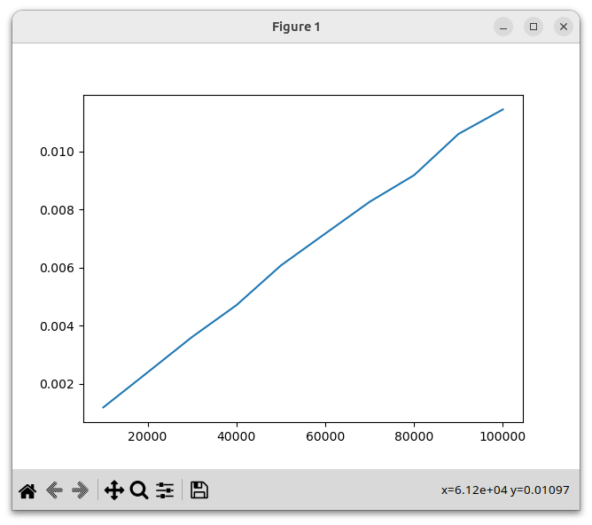
To see this graphically, let's write code that builds a DynArray with 100,000 elements. After every 10,000 elements, we'll measure the time in seconds taken so far. At the end, we'll plot these times:
import time
import matplotlib.pyplot as plt

class DynArray:
  ...

d = DynArray()
start = time.time()
xs = range(10_000, 110_000, 10_000)
ys = []
for x in xs:
    print(x)
    # grow the array to size x
    while d.length() < x:
        d.add(0)
    ys.append(time.time() - start)

plt.plot(xs, ys)
plt.show()
Here is the result:

We can see that the running time grows quadratically, which is unfortunate.
We can make a tiny change to the add() method to dramatically improve the algorithmic running time. When we grow the array, instead of adding a constant number of elements, let's double its size. The add() method will now look like this:
    def add(self, x):
        if self.count == len(self.a):               # array self.a is full
            self.a = self.a + self.count * [None]   # expand array
        self.a[self.count] = x
        self.count += 1
Now let's reconsider the running time of the loop we wrote above. Here is its again:
d = DynArray()
for i in range(N):
    d.add(i)
The total time for all the resize operations will now be O(10 + 20 + 40 + 80 + … + N).
Now, we have previously seen (e.g. in our discussion of binary trees) that 1 + 2 + 4 + 8 + ... + 2k = 2k + 1 - 1. Or, if we let M = 2k, we see that 1 + 2 + 4 + 8 + ... + M = 2M - 1 = O(M). And so the total resize time is
O(10 + 20 + 40 + 80 + … + N) = 10 ⋅ O(1 + 2 + 4 + 8 + … + (N / 10)) = 10 ⋅ O(N / 10) = O(N)
And so the time for each of the N calls to add() will be O(1) on average. That's an enormous improvement.
With this change, let's regenerate our performance graph:
We see that this implementation is dramatically faster, and the running time now grows linearly.
In fact Python's built-in list type is implemented in a similar fashion. That is why calls to Python's append() method run in O(1) on average. (If you really want to understand how Python lists work, you can study the source code for lists inside the CPython interpreter, which is written in C.)