Recursion is one of the most fundamental concepts we've learned about in Programming 1 and Introduction to Algorithms. In this lecture we'll look at some more problems that we can solve recursively, and expand our knowledge of how to solve recurrences.
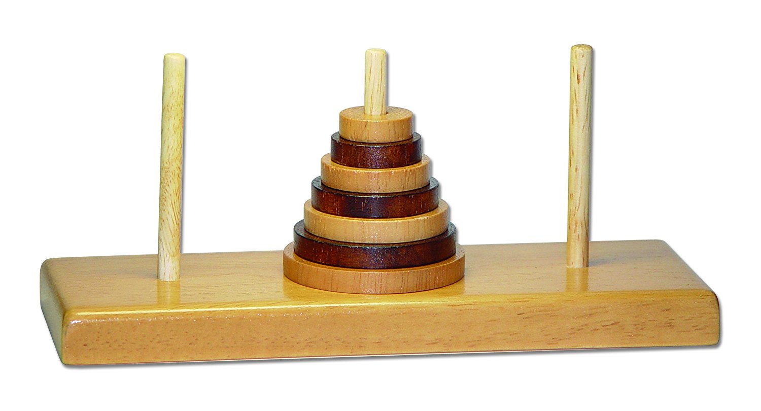
The Tower of Hanoi is a well-known puzzle that looks like this:
The puzzle has 3 pegs and a number of disks of various sizes. The player may move disks from peg to peg, but a larger disk may never rest atop a smaller one. Traditionally all disks begin on the leftmost peg, and the goal is to move them to the rightmost.
Supposedly in a temple in the city of Hanoi there is a real-life version of this puzzle with 3 rods and 64 golden disks. The monks there move one disk each second from one rod to another. When they finally succeed in moving all the disks to their destination, the world will end!
The world has not yet ended, so we can write a program that solves a version of this puzzle with a smaller number of disks. We want our program to print output like this:
move disk 1 from 1 to 2
move disk 2 from 1 to 3
move disk 1 from 2 to 3
move disk 3 from 1 to 2
…
To solve this puzzle, the key insight is that a simple recursive algorithm will do the trick. To move a tower of disks 1 through N from peg A to peg B, we can do the following:
Move the tower of disks 1 through N-1 from A to C.
Move disk N from A to B.
Move the tower of disks 1 through N-1 from C to B.
The program below implements this algorithm:
# move tower of n disks from fromPeg to toPeg
def hanoi(n, fromPeg = 1, toPeg = 3):
  if n == 0:
    return

  other = 6 - fromPeg - toPeg
  hanoi(n - 1, fromPeg, other)
  print(f'move disk {n} from {fromPeg} to {toPeg}')
  hanoi(n - 1, other, toPeg)
Notice that above the base case is when n == 0, in which case we don't need to print anything at all. As usual, the smallest possible base case leads to the simplest code.
We can compute the exact number of moves required to solve the puzzle using the algorithm above. If M(n) is the number of moves to move a tower of height n, then we have the recurrence
M(0) = 0
M(n) = 2
⋅ M(n – 1) + 1
The solution to this recurrence is, exactly,
M(n) = 2n – 1
Similarly, the running time of our program above follows the recurrence
T(n) = 2 ⋅ T(n–1) + O(1)
And the program runs in time T(n) = O(2n).
It will take 264 - 1 seconds for the monks in Hanoi to move the golden disks to their destination tower. That is far more than the number of seconds that our universe has existed so far.
As an exercise, you may wish to implement a graphical animation of the Tower of Hanoi's solution using Tkinter or Pygame.
Recall that when we studied mergesort, we found that its running time follows this recurrence:
T(N) = 2 T(N / 2) + O(N)
We also found that quicksort follows the same recurrence if we are perfectly lucky in our choice of pivots, i.e. each partition operation splits a subarray of values exactly in half.
If the recurrence above is not obvious to you, you should review our notes on mergesort and quicksort from an earlier lecture.
Also recall that we solved the recurrence above by expanding it into a recursion tree that looked like this:
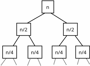
We can see algebraically that the recurrence will expand into this tree:
T(N) = O(N) + 2 T(N / 2)
= O(N) + 2[O(N / 2) + 2 T(N / 4)]
= O(N) + 2[O(N / 2) + 2 [O(N / 4) + ...]]
We know that O(N) means a function that is eventually bounded by C · N for some constant C. All the occurrences of big O in the expansion above will have the same constant factor C. We have not bothered to include this constant factor in the tree nodes above.
We can easily see that the sum of every row in the tree above will be N. The tree has log2 N levels, since we must divide by 2 that many times to reach the value 1. And so we have T(N) = O(N log N).
We may use the same recursion tree technique to solve many other recurrences. For example, suppose that in quicksort every partition operation divides a subarray of values into two partitions P and Q, where P contains 2/3 of the values in the subarray and Q contains the remaining 1/3. Then we will have the recurrence
T(N) = T(2 N / 3) + T(N / 3) + O(N)
That will expand into a tree that looks like this:
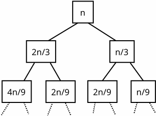
Once again we see that the sum of all values in each of the topmost rows of the tree is n. However, in this tree not all leaves will be at the same level. That's because when we descend rightward and multiply by 1/3 at each step, we will reach the value 1 more quickly than when we descend leftward and multiply by 2/3 at each step. So some lower rows of the tree will be incomplete, i.e. there will be no nodes in the rightmost part of some rows. In those rows the sum of all values will be less than n. The total number of rows (including incomplete rows) will be log3/2 n, which is the number of steps it will take to reach 1 when descending to the left. But then the total of all values in the tree will be less than n · log3/2 n, so we still have T(N) = O(N log N).
Generalizing the previous result, suppose that in each partition P contains some fraction f of the values in the subarray and Q contains the remaining (1 - f), where f is a constant with 0 < f < 1. Then T(N) = T(f N) + T((1 - f) N) + O(N), and we will still have T(N) = O(N log N).
Consider this problem: given an unsorted array with N elements, we wish to find the smallest element. The solution is trivial: we walk over the elements, always remembering the smallest element we've seen so far. This will run in O(N).
Now suppose that we wish to find the second smallest element in the array. This is still easy: we traverse the array, always remembering the two smallest elements that we've seen so far. At each step, we update those elements by comparing them with the next array element. That update can be performed in O(1), so the total time will be O(N). Implementing this is an easy exercise.
Now suppose that the array has an odd number of elements, and we wish to find the median value in the array. This is significantly harder. As a trivial solution, we may sort the array, then choose the element in the middle position after that. This will take O(N log N), which is the cost of the sort. Can we do better?
The quickselect algorithm will let us find the median value, or in fact the kth smallest value for any k, in expected linear time. Like quicksort, it uses a function that can divide a subarray into two partitions around a pivot element. We saw earlier that we can write this function using the Hoare partitioning algorithm:
# We are given an unsorted range a[lo:hi] to be partitioned, with
# hi - lo >= 2 (i.e. at least 2 elements in the range).
#
# Choose a pivot value p, and rearrange the elements in the range into
# two partitions p[lo:k] (with values <= p) and p[k:hi] (with values >= p).
# Both partitions must be non-empty.
#
# Return k, the index of the first element in the second partition.
def partition(a, lo, hi):
    # Choose a random element as the pivot, avoiding the first element
    # (see the discussion below).
    p = a[randrange(lo + 1, hi)]

    i = lo
    j = hi - 1

    while True:
        # Look for two elements to swap.
        while a[i] < p:
            i += 1
        while a[j] > p:
            j -= 1

        if j <= i:             # nothing to swap
            return i

        a[i], a[j] = a[j], a[i]
        i += 1
        j -= 1
The idea behind quickselect is simple. Suppose that we are looking for the i-th smallest element in an array a of N elements. As usual in computer science we'll count from 0, so if i = 0 we want the smallest element, if i = 1 we want the second smallest element, and so on. Equivalently, we're looking for the element that would be a[i] if we were to first sort the array a. (Once again, we don't actually want to sort a since that would be too slow.) We will call the partition function to divide a into two partitions P and Q. Suppose that P contains k elements and Q contains the remaining (N - k) elements. All elements in P will be less than or equal to all elements in Q. So if i < k, then the value we are looking for is in the partition P, and we can recursively call the function looking for the i-th elements of P. Otherwise, the value we are looking for is in the partition Q, and we can recursively call the function looking for the (i - k)-th element of Q.
To implement this algorithm efficiently in Python, we'll need to write the function so that it can find the i-th smallest element in a subarray a[lo:hi] for any given values of 'lo' and 'hi'. Here is an implementation:
# Return the i-th smallest element of a[lo:hi], where i starts from 0.
def quickselect(a, lo, hi, i):
    if hi - lo < 2:
        return a[lo]

    k = partition(a, lo, hi)
    if i < k - lo:
        return quickselect(a, lo, k, i)
    else:
        return quickselect(a, k, hi, i - (k - lo))

def median(a):
    return quickselect(a, 0, len(a), (len(a) - 1) // 2)
We have presented a recursive solution. However notice that quickselect() only calls itself once, so alternatively we could easily write the function iteratively if we like.
How long will this function take to run? In the worst case, the partition function will always partition a subarray of length N into partitions of length 1 and (N - 1), and we will always recurse into the longer of these partitions. Then the function will recurse N times until it reaches a subarray with a single element. The total time for all the partition operations will be O(N + (N - 1) + ... + 1) = O(N2).
However, just as in quicksort the average case will be much better. In fact this function will run in O(N) on average. Here is an informal argument to show that. On each recursive step there is a 50% chance that we will recurse into the smaller partition, in which case our subarray size has dropped by a factor of at least 2. So suppose that this happens 50% of the time, and that (conservatively) on the other recursive steps the subarray size does not decrease at all. Then the total cost of the partition operations will be less than O(N + N + N / 2 + N / 2 + N / 4 + N / 4 + ...) = O(N). You may see a more formal proof of this fact in a more advanced class such as ADS 1 or ADS 2.
The algorithm we have described is simple, and runs in O(N) on average and in O(N2) in the worst case. In fact it is possible to do even better: a variation of this algorithm will run in O(N) even in the worst case! That variation is called the "median of medians" algorithm, and you may see it in a more advanced class.