Week 8: Notes

dictionaries

We have already seen several abstract data types: stacks, queues, and sets. Another abstract data type is a dictionary (also called a map or associative array), which maps keys to values. It provides these operations:

d.set(key, value)

Add a new (key, value) pair, or update an existing key if present.

d.remove_key(key)

Remove a key and its associated value.

d.lookup(key)

Look up a key and return its associated value, or None if absent.

A dictionary cannot contain the same key twice. In other words, a dictionary associates a key with exactly one value.

This type should be familiar, since we have used Python's dictionaries, which are an implementation of this abstract type.

implementing a dictionary

In general, given any implementation of the set abstract data type, it is usually easy to modify it to implement a dictionary.

For example, we can use a binary search tree to implement a dictionary. To do so, we only need to make a small change to the binary search tree code we saw last week: now each node will store a key-value pair. In Python, our Node class will look like this:

class Node:
    def __init__(self, key, val, left, right):
        self.key = key
        self.val = val
        self.left = left
        self.right = right

The lookup() operation will be similar to the set operation contains(): it will search the tree for a node with the given key; if found, it will return the corresponding value. The dictionary operations set() and remove_key() will also be similar to the set operations add() and remove(). I won't implement these operations here; if you like, you can write them yourself as an easy exercise.

dynamic arrays

Let's consider another abstract data type, namely a dynamic array. A dynamic array d has these operations:

d.add(x)

Append a value to the array.

d.get(i)

Retrieve the value at the given index.

d.set(i, x)

Set the value at the given index.

This interface probably looks familiar, since a Python list is a dynamic array!

In lower-level languages such as C an array typically has a fixed size. Let's now implement a dynamic array in Python, using only fixed-size arrays. That means that in our implementation we can allocate an array using an expression such as '10 * [None]', but we may not call the append() method to expand an existing array.

We'll use a class with two attributes: a fixed-size array a plus an attribute n that indicates how many elements in the array are currently in use. Each time we add an element to the dynamic array, we first check if the underlying array a is full. If so, we'll allocate a new array that is 10 elements larger, and copy all elements from the old array to the new array.

Here is our implementation:

class DynArray:
    def __init__(self):
        self.a = 10 * [None]
        self.count = 0
    
    def get(self, i):
        return self.a[i]
    
    def set(self, i, x):
        self.a[i] = x

    def length(self):
        return self.count

    def add(self, x):
        if self.count == len(self.a):       # array self.a is full
            self.a = self.a + 10 * [None]   # expand array
        self.a[self.count] = x
        self.count += 1

Note that the line with the comment "expand array" above does not expand the original array self.a. The + operator allocates a new array, so it is equivalent to this code:

b = (self.count + 10) * [None]   # allocate an array with 10 extra elements
for i in range(self.count):
    b[i] = self.a[i]
self.a = b

Our class works:

>>> d = DynArray()
>>> for x in range(1, 1001):
...   d.add(x)
... 
>>> d.get(100)
101
>>> d.get(500)
501

Now suppose that we create a DynArray and add N elements in a loop:

d = DynArray()
for i in range(N):
    d.add(i)

How long will this take, as a big-O function of N?

The total time will be the time for all the resize operations, plus the extra work done by the last two lines in the add() method. The extra work takes O(1) per element added, so the total time of the extra work is O(N).

A single resize operation from size S to size S + 10 must allocate an array of size S + 10, then copy S elements to the new array. Both of these operations take time O(S), so the total time for a single resize operation from size S is O(S). Then the total time for all the resize operations will be

O(10 + 20 + 30 + … + N) = O(1 + 2 + 3 + … + (N / 10)) = O((N / 10)²) = O(N²).

So the total time for the loop to run will be O(N) + O(N²) = O(N²). And so the average time for each of the N calls to add() will be O(N). That's pretty slow.

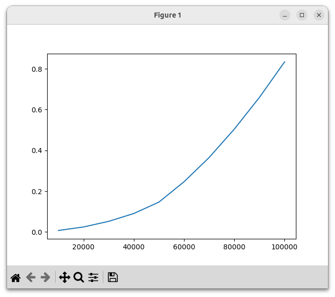
To see this graphically, let's write code that builds a DynArray with 100,000 elements. After every 10,000 elements, we'll measure the time in seconds taken so far. At the end, we'll plot these times:

import time
import matplotlib.pyplot as plt

class DynArray:
  ...
    
d = DynArray()
start = time.time()
xs = range(10_000, 110_000, 10_000)
ys = []
for x in xs:
    print(x)
    # grow the array to size x
    while d.length() < x:
        d.add(0)
    ys.append(time.time() - start)

plt.plot(xs, ys)
plt.show()

Here is the result:

We can see that the running time grows quadratically, which is unfortunate.

We can make a tiny change to the add() method to dramatically improve the algorithmic running time. When we grow the array, instead of adding a constant number of elements, let's double its size. The add() method will now look like this:

    def add(self, x):
        if self.count == len(self.a):               # array self.a is full
            self.a = self.a + self.count * [None]   # expand array
        self.a[self.count] = x
        self.count += 1

Now let's reconsider the running time of the loop we wrote above. Here is its again:

d = DynArray()
for i in range(N):
    d.add(i)

The total time for all the resize operations will now be O(10 + 20 + 40 + 80 + … + N).

Now, we have previously seen (e.g. in our discussion of binary trees) that 1 + 2 + 4 + 8 + ... + 2^k = 2^{k + 1} - 1. Or, if we let M = 2^k, we see that 1 + 2 + 4 + 8 + ... + M = 2M - 1 = O(M). And so the total resize time is

O(10 + 20 + 40 + 80 + … + N) = 10 ⋅ O(1 + 2 + 4 + 8 + … + (N / 10)) = 10 ⋅ O(N / 10) = O(N)

And so the time for each of the N calls to add() will be O(1) on average. That's an enormous improvement.

With this change, let's regenerate our performance graph:

We see that this implementation is dramatically faster, and the running time now grows linearly.

In fact Python's built-in list type is implemented in a similar fashion. That is why calls to Python's append() method run in O(1) on average. (If you really want to understand how Python lists work, you can study the source code for lists inside the CPython interpreter, which is written in C.)

hash functions

A hash function maps values of some type T to integers in a fixed range. Often we will want a hash function that produces values in the range 0 .. (N – 1), where N is a power of 2. Hash functions are very useful, and are a common building block in programming and also in theoretical computer science.

In general, there may be many more possible values of T than integers in the output range. (For example, if T is the type of strings, there is an infinite number of possible values.) This means that hash functions will inevitably map some distinct input values to the same output value; this is called a hash collision. A good hash function will produce relatively few collisions in practice. In other words, even if two input values are similar to each other, they should be unlikely to have the same hash value. An ideal hash function will produce hash collisions in practice no more often than would be expected if it were producing random outputs.

Our immediate motivation for hash functions is that we'll use them to build hash tables, which we'll see in the next lecture. A hash table, like a binary tree, can be used to implement a set. Broadly speaking, if we have some values (e.g. strings) that we want to store in a hash table, we'll divide the values into some number K of distinct buckets. To decide which bucket to place a value V in, we'll compute a hash of the value V, producing an integer n, and will then compute a bucket number (n mod K). By dividing the values in this way, we can implement lookup operations efficiently. We want a hash function that produces numbers that are roughly evenly distributed among the range 0 .. (N - 1), so that our buckets will contain roughly equal numbers of values. That's all we need to know about hash tables for the moment; we'll discuss them in more detail in the next lecture.

hashing strings

In practice, we will very often want a hash function that takes strings as input. As a starting point, suppose that we want a hash function that takes strings of characters with ordinal values from 0 to 255 (i.e. with no fancy Unicode characters) and produces hash values in the range 0 ≤ v < N for some constant N.

As one simple idea, we could add the ordinal values of all characters in the input string, then take the result mod N. For example, with N = 2³²:

# Generate a hash code in the range 0 .. 2^32 – 1.
def my_hash(s):
    return sum([ord(c) for c in s]) % (2 ** 32)

This is a poor hash function. If the input strings are short, then the output values will always be small integers. Furthermore, two input strings that contain the same set of characters (a very common occurrence) will hash to the same number.

Here is one way to construct a better hash function, called modular hashing. Given any string s, consider it as a series of digits forming one large number H. For example, since our characters have ordinal values in the range from 0 to 255, we can imagine them to be digits in base 256. This will give us an integer H, and then we can compute H mod N, producing a hash value in the range from 0 to N – 1.

Here is Python code that implements this idea, with N = 2³²:

# Generate a hash code in the range 0 .. 2^32 – 1
def my_hash(s):
    h = 0
    for c in s:
        d = ord(c)    # 0 .. 255
        h = 256 * h + d
    return h % (2 ** 32)

As you can see, this code is using the algorithm for combining digits in any base that we learned in one of the very first lectures of this class!

As we wrote above, a good hash function will allow us to distribute a set of values into a set of K buckets, with roughly the same number of values in each bucket. Specifically, we'll place each value v into the bucket h(v) mod K, where h is the hash function. To test this hash function, let's place all the words in this poem into 64 buckets, then plot the result.

import matplotlib.pyplot as plt

def my_hash(s):
  ...

with open('poem.txt') as f:
    words = { word for line in f for word in line.split() }

NUM_BUCKETS = 64
buckets = [0] * NUM_BUCKETS
for word in words:
    h = my_hash(word)
    b = h % NUM_BUCKETS
    buckets[b] += 1

plt.bar(range(64), buckets)
plt.show()

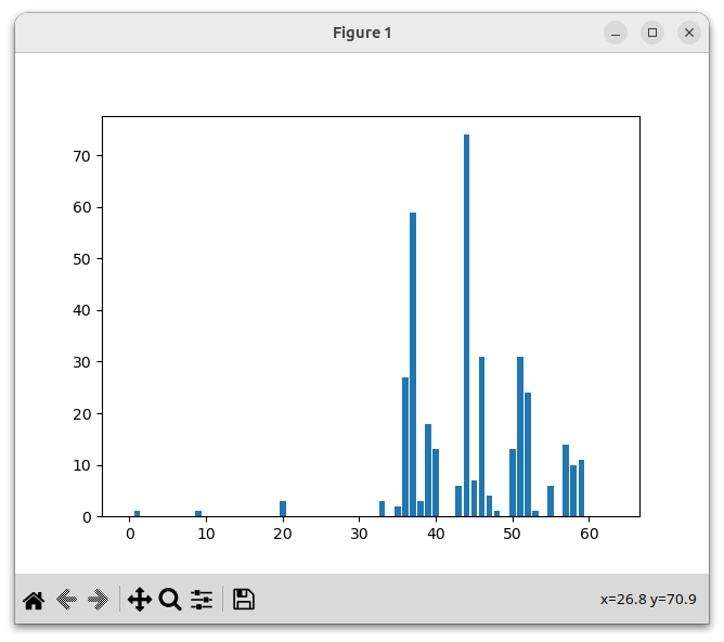
We see that the result is poor: the values are not evenly distributed at all.

In fact, our hash function often maps similar strings to the same hash value:

>>> my_hash('bright')
1768384628
>>> my_hash('light')
1768384628
>>> my_hash('night')
1768384628

The problem is that if we have a number H in base 256, then H mod 2³² is exactly the last four digits of the number, because 2³² = 256⁴. If that's not obvious, consider the same phenomenon in base 10: 2,276,345 mod 10,000 = 6,345, because 1,000 = 10⁴.

And so this hash function only depends on the last four characters in the string. By the way, here's another way to think about this: for any number N in binary, N mod 2³² gives you the last 32 bits of the number, and the last 32 bits depend on only the last four 8-bit characters.

In our poem hashing example above, we computed a bucket number h(v) mod K, where K = 64. This makes the problem even worse. If H is the value of the string as a base-256 number, then we are computing ((H mod 2³²) mod 64), which is the same as H mod 64 (since 2³² is divisible by 64). And because 256 is divisible by 64, that value depends on only the last character of the string:

>>> my_hash('watermelon') % 64
46
>>> my_hash('man') % 64
46
>>> my_hash('n') % 64
46

To put it differently, we're taking only the last 6 bits of the number H (since 64 = 2⁶), which depend only on the last (8-bit) character of the input string.

How can we improve the situation? Generally speaking, if B is the base of our digits (e.g. B = 256 here), and N is the size of the hash function output range (e.g. N = 2³² here), then we will probably get the best hash behavior if B and N are relatively prime, i.e. have no common factors. So if we want a better hash function, we must change B or N. Assuming that we want to produce values in a certain fixed range, we'd like to keep N as it is. So let's change B. In fact we'd like B to be larger anyway, so that we can process strings with Unicode characters, whose ordinal values might be as high as 10FFFF₁₆ = 1,114,112.

In fact it will probably be best if B is not too close to a power of 2 (for number-theoretic reasons that we won't go into here). A good choice for B might be the prime number 1,000,003, which is used in various popular implementations of hash functions, including Python's own built-in hash function. (Actually this is less than the highest possible Unicode value, so this might cause poor behavior if we have some Unicode characters with values higher than 1,000,003. Such characters are rare, so let's not worry about that.) To be clear, we will now consider the input string to be a series of digits in base 1,000,003!

Let's modify our hash function to use this value of B:

# Generate a hash code in the range 0 .. 2^32 - 1
def my_hash(s):
    h = 0
    for c in s:
        d = ord(c)
        h = 1_000_003 * h + d
    return h % (2 ** 32)

Now we get distinct values for the strings we saw above:

>>> my_hash('bright')
2969542966
>>> my_hash('light')
1569733066
>>> my_hash('night')
326295660

Let's now rerun the experiment we ran above, in which we use the hash function to place all words from a poem into one of 64 hash buckets:

This looks like a much better distribution.

Now, a disadvantage of our latest version of my_hash() is that it computes an integer h that will be huge if the input string is large, since it encodes all of the characters in the string. That may be inefficient, and in fact many programming languages don't support large integers of this sort.

However, we can make a tiny change to the code so that it will compute the same output values, but be far more efficient. Rather than taking the result mod 2³² at the end, we can perform it at every step of the calculation:

# Generate a hash code in the range 0 .. 2^32 - 1
def my_hash(s):
    h = 0
    for c in s:
        d = ord(c)    # 0 .. 255
        h = (1_000_003 * h + d) % (2 ** 32)
    return h

This function still computes the same hash values that the previous version did:

>>> my_hash('bright')
2969542966
>>> my_hash('light')
1569733066
>>> my_hash('night')
326295660

Why does this trick work? A useful mathematical fact is that if you're performing a series of additions and multiplications and you want the result mod N, you can actually perform a (mod N) operation at any step along the way, and you will still get the same result! I won't prove this statement here, but ultimately it is true because of this fact, which you may have seen in your math classes: if

a ≡ b (mod N) and c ≡ d (mod N)

then

a + c ≡ b + d (mod N)

and

a ⋅ c ≡ b ⋅ d (mod N) .

This fact is especially useful in lower-level languages such as C that have fixed-size integers, because arithmetic operations in those languages automatically compute the result mod N for some fixed N (where typically N = 2³² or N = 2⁶⁴).

hashing other data types

Of course, we may want to hash other data types, such as pairs, or lists. In theory, we could convert any value of any type to a string representation such as "[32, 57, 88]", then apply the string hashing function we wrote above. However that would not be too efficient. As a better idea, if we can convert a value of any other type to a large integer, then we can use the same modular hashing technique we saw above. For example, if we want to compute a hash code for a list of integers, we might first take each integer in the list mod P (where P is a large fixed prime), then concatenate all the bits of the resulting integers together (which is the same as considering it to be a number written in a series of digits in base P), then take that number mod N. I won't go into details about this here, but the same general idea will apply to most data types.