In last week's lecture we learned about two basic sorting algorithms: bubble sort and selection sort. We found that each of them runs in O(N2) in the best and worst cases.
Insertion sort is another fundamental
sorting algorithm. An insertion
sort loops through array elements from left to right. For each
element a[i], we
first "lift" the element out of the array by saving
it in a temporary variable t. We then walk leftward from
i; as we go, we find all elements to the left of a[i]
that are greater than a[i] and shift them rightward one
position. This makes room so that we can insert a[i] to
the left of those elements. And now the subarray a[0..i]
is in sorted order. After we repeat this for all elements in turn,
the entire array is sorted.
Here is an animation of insertion sort in action.
Here is a Python implementation of insertion sort:
def insertion_sort(a):
    n = len(a)
    for i in range(n):
        t = a[i]
        j = i - 1
        while j >= 0 and a[j] > t:
            a[j + 1] = a[j]
            j -= 1
        a[j + 1] = t
What is the running time of insertion sort on an array with N elements? The worst case is when the input array is in reverse order. Then to insert each value we must shift elements to its left, so the total number of shifts is 1 + 2 + … + (N – 1) = O(N2). If the input array is ordered randomly, then on average we will shift half of the subarray elements on each iteration. Then the time is still O(N2).
In the best case, the input array is already sorted. Then no elements are shifted or modified at all and the algorithm runs in time O(N).
Insertion sort will perform well even when the array is mostly but not completely sorted. For example, suppose that we run insertion sort on an array that is almost sorted, but two adjacent elements are out of order, e.g.
2 7 9 15 13 18 20 22
When the sort processes most elements, no elements need to shift. When it encounters the two elements that are out of order, it will need to shift one of them, which takes O(1). The total time will be O(N) + O(1) which is still O(N).
Now suppose that the input is almost sorted, but the first and last elements have been swapped, e.g.
22 7 9 13 15 18 20 2
In this case as the sort encounters each element before the last it will need to shift a single element, which takes O(1). When it encounters the last element, it will need to shift it all the way back to the front, which takes O(N). The total time of all these shifts will be (N - 2) * O(1) + O(N) = O(N) + O(N) = O(N). So even in this case the sort will take linear time.
In fact, if we take a sorted array and swap any two elements that we like (or indeed, even make a constant number of such swaps), insertion sort will still sort the resulting array in linear time!
In summary, insertion sort has the same worst-case asymptotic running time as bubble sort and selection sort, i.e. O(N2). However, insertion sort has a major advantage over bubble sort and selection sort in that it is adaptive: when the input array is already sorted or nearly sorted, it runs especially quickly.
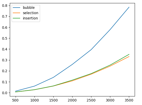
Let's extend our previous plot by adding insertion sort:
We see that on random data, selection sort and insertion sort behave quite similarly.
Now let's compare the running times of these algorithms on data that is already sorted:

As we can see, in this situation insertion sort is enormously faster. As we discussed above, with sorted input it runs in O(N).
We have already studied how to analyze the running time of iterative functions, i.e. functions that use loops. We'd now like to do the same for recursive functions.
To analyze any recursive function's running time, we perform two steps. First, we write a recurrence, which is an equation that expresses the function's running time recursively, i.e. in terms of itself. Second, we solve the recurrence mathematically. In this class, we will generally derive solutions to recurrences somewhat informally. (In ADS 1 next semester, you will study this topic with more mathematical rigor.)
For example, consider this simple recursive function:
def fun1(n):
    if n == 0:
        return 0

    return n * n + fun1(n - 1)
The function computes the sum 12 + 22 + … + n2, using recursion to perform its task.
Let's write down a recurrence that expresses this
function's running time. Let T(N) be the time to run fun1(N).
The function performs a constant amount of work outside the recursive
call (since we assume that arithmetic operations run in constant
time). When it calls itself recursively, n decreases by 1. And so we
have the equations
T(0) = O(1)
T(N) = T(N - 1) + O(1)
Now we'd like to solve the recurrence. We can do so by expanding it algebraically. O(1) is some constant C. We have
T(N)
= C + T(N - 1)
= C + C + T(N – 2)
= …
= C + C +
... + C (N times)
=
N · C
= O(N)
The function runs in linear time. That's not a surprise, since an iterative loop to sum these numbers would also run in O(N).
When we write recurrences from now on, we will usually not bother to write a base case 'T(0) = O(1)', and will only write the recursive case, e.g. 'T(N) = T(N - 1) + O(1)'.
Now consider this function:
def fun2(n):
    if n == 0:
        return 0

    s = 0
    for i in range(n):
        s += n * i

    return s + fun2(n – 1)
The 'for' loop will run in O(N), so the running time will follow this recurrence:
T(N) = T(N – 1) + O(N)
We can expand this algebraically. O(N) is CN for some constant C, so we have
T(N)
= CN + T(N – 1)
= CN + C(N – 1) + T(N – 2)
= CN + C(N
– 1) + C(N - 2) + T(N - 3)
= …
= C(N + (N – 1) + …
+ 1)
= C(O(N2))
= O(N2)
As another example, consider this recursive function that computes the binary representation of an integer:
def fun3(n):
    if n == 0:
        return ''

    d = n % 2
    return fun3(n // 2) + str(d)
The work that the function does outside the recursive calls takes constant time, i.e. O(1). The function calls itself recursively at most once. When it calls itself, it passes the argument (n // 2). So we have
T(N) = T(N / 2) + O(1)
To solve this, let's again observe that O(1) is some constant C. We can write
T(N)
= C + T(N / 2)
= C + C + T(N / 4)
= …
= C + C + ...
+ C (log2(N)
times)
= C log2(N)
=
O(log N)
Next, consider this function:
def fun4(n):
    if n == 0:
        return 0

    s = 0
    for i in range(n):
        s += i * i

    return s + fun4(n // 2)
The running time follows this recurrence:
T(N) = T(N / 2) + O(N)
Let O(N) = CN. Then we have
T(N)
= CN + T(N / 2)
= CN + C(N / 2) + T(N / 4)
= CN + C(N / 2)
+ C(N / 4) + T(N / 8)
…
= C(N + N / 2 + N / 4 + …)
=
C(2N)
= O(N)
These recurrences were relatively easy to solve, since they arose from recursive functions that call themselves at most once. When a recursive function calls itself twice or more, the resulting recurrence may not be quite so easy. For example, recall the Fibonacci sequence:
1, 1, 2, 3, 5, 8, 13, 21, ...
Its definition is
F1 = 1
F2 = 1
Fn = Fn - 1 + Fn - 2 (n ≥ 3)
We may directly translate this into a recursive Python function:
def fib(n):
    if n <= 2:
        return 1

    return fib(n - 1) + fib(n - 2)
Let T(N) be the running time of this function on an integer N ≥ 3. We have
T(N) = O(1) + T(N - 1) + T(N - 2)
Omitting the term O(1), we see that T(N) > T'(N), where
T'(N) = T'(N - 1) + T'(N - 2)
Now observe that this recurrence for T'(N) is just the same as for the Fibonacci numbers Fn themselves! This shows that T(N) is at least O(Fn).
Now, it can be shown that the Fibonacci numbers increase exponentially, and so T(N) also grows exponentially, i.e. faster than any polynomial function such as N2 or N4.
Why is this function so inefficient? The essential problem is that it will perform the same subcomputations over and over. For example, if we call fib(40), that will recursively call both fib(39) and fib(38). Those functions will make further recursive calls, and so on:
fib(40)
= fib(39) + fib(38)
= (fib(38) + fib(37)) + (fib(37) + fib(36))
= ...
The two instances of fib(37) above are separate repeated computations. As this tree expands, smaller subcomputations such as fib(20) and fib(10) will occur an enormous (exponential) number of times.
We could make this function much faster by caching the results of subcomputations so that each subcomputation occurs only once. We'll discuss this topic more in Programming 2 in next semester. For the moment, the important point is that recursion, though powerful, lets us easily write functions that will take exponential time to run.
As a step toward our next sorting algorithm, suppose that we have two arrays, each of which contains a sorted sequence of integers. For example:
a = [3, 5, 8, 10, 12]
b = [6, 7, 11, 15, 18]
And suppose that we'd like to merge the numbers
in these arrays into a single array c
containing all of the numbers in sorted order.
A simple algorithm will
suffice. We can use integer variables i
and j
to point to members of a
and b,
respectively. Initially i
= j
= 0. At each step of the merge, we compare a[i]
and b[j].
If a[i] < b[j],
we copy a[i]
into the destination array, and increment i. Otherwise we copy b[j]
and increment j. The entire process will run in linear time, i.e. in
O(N) where N = len(a) + len(b).
Let's write a function to accomplish this task:
# Merge sorted arrays a and b into c, given that
# len(a) + len(b) = len(c).
def merge(a, b, c):
    i = j = 0     # index into a, b

    for k in range(len(c)):
        if j == len(b):      # no more elements available from b
            c[k] = a[i]      # so we take a[i]
            i += 1
        elif i == len(a):    # no more elements available from a
            c[k] = b[j]      # so we take b[j]
            j += 1
        elif a[i] < b[j]:
            c[k] = a[i]      # take a[i]
            i += 1
        else:
            c[k] = b[j]      # take b[j]
j += 1We can use this function to merge the arrays a and b mentioned above:
>>> a = [3, 5, 8, 10, 12]
>>> b = [6, 7, 11, 15, 18]
>>> c = (len(a) + len(b)) * [0]
>>> merge(a, b, c)
>>> c
[3, 5, 6, 7, 8, 10, 11, 12, 15, 18]
>>>
We now have a function that merges two sorted arrays. We can use this as the basis for implementing a sorting algorithm called merge sort.
Merge sort has a recursive structure. To sort an array of n elements, it divides the array in two and recursively merge sorts each half. It then merges the two sorted subarrays into a single sorted array.
For example, consider merge sort’s operation on this array:

Merge sort splits the array into two halves:

It then sorts each half, recursively.

Finally, it merges these two sorted arrays back into a single sorted array:

Here's an implemention of merge sort, using our merge() function from the previous section:
def merge_sort(a):
    if len(a) < 2:
        return

    mid = len(a) // 2

    left = a[:mid]      # copy of left half of array
    right = a[mid:]     # copy of right half

    merge_sort(left)
    merge_sort(right)

    merge(left, right, a)
Let's add merge sort to our performance graph, showing the time to sort random input data:
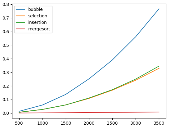
As we can see, merge sort is enormously faster than any of the other sorting methods that we have seen. Let's draw a plot showing the performance of only merge sort, with larger input sizes:
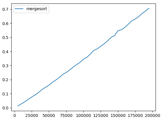
The performance looks nearly linear.
What is the actual big-O running time of merge
sort? In the code above, the helper function merge runs
in time O(N), where N is the length of the array c. The array slice
operations a[:mid] and a[mid:] also take
O(N). So if T(N) is the time to run merge_sort on an
array with N elements, then we have
T(N) = 2 T(N / 2) + O(N)
We have not seen this recurrence before. Let O(N) = CN for some constant C. We have T(N) = 2 T(N / 2) + CN, so we know that T(N) is the sum of all the terms here:

Let's expand each leaf using the same equation:

And again:

We can continue this process until we reach the base case T(1) = O(1). We'll end up with a tree with log2 N levels, since that's how many times we must divide by 2 to reach 1. Notice that the sum of the values on every level is CN: we have 2(C / 2) = 4 (C / 4) = N, for instance. So the total of all terms on all levels will be CN(log2 N). This informal argument has shown that
T(N) = O(N log N)
By the way, the tree above also illustrates the structure of the recursive calls that happen as the mergesort proceeds.
For large N, O(N log N) is much faster than O(N2), so mergesort will be far faster than insertion sort or bubble sort. For example, suppose that we want to sort 1,000,000,000 numbers. And suppose (somewhat optimistically) that we can perform 1,000,000,000 operations per second. An insertion sort might take roughly N2 = 1,000,000,000 * 1,000,000,000 operations, which will take 1,000,000,000 seconds, or about 32 years. A merge sort might take roughly N log N ≈ 30,000,000,000 operations, which will take 30 seconds. This is a dramatic difference!
We've
seen that merge sort is quite efficient. However, one potential
weakness of merge sort is that it will not run in
place:
it requires extra memory beyond that of the array that we wish to
sort. That's because the merge step won't run in place: it requires
us to merge two arrays into an array that is held in a different
region of memory. So any implementation of merge sort must make a
second copy of data at some point. (Ours does so in the lines 'left
= a[:mid]'
and 'right = a[mid:]',
since an array slice in Python creates a copy of a range of
elements.)