Suppose that we want to search for a value (sometimes called the “key”) in an unsorted array of values. All we can do is to scan the array sequentially, looking for the value we want. Here's a function that will do that:
# Find the value k in the array a and return its index.
# Return -1 if not found.
def find(a, k):
    for i in range(len(a)):
        if a[i] == k:
            return i

    return -1
This is a trivial algorithm. Suppose that the input array has N elements. The algorithm will run in O(N) in the worst case, since it might need to scan the entire array, and in O(1) in the best case, since it might find the value immediately, even if the array is large.
The Python expression 'k in a' performs this sort of
sequential search, so it will also run in O(N) in the worst case and
O(1) in the best. (Later in this course we'll see other sorts of data
structures for which in will be far more efficient.)
Now suppose that we want to search for a key value in a sorted array. We can use a fundamental algorithm called binary search to find the key efficiently.
Binary search is related to a well-known number-guessing game. In that game, one player thinks of a number N, say between 1 and 1,000. If we are trying to guess it, we can first ask "Is N greater than, less than, or equal to 500?" If we learn that N is greater, then we now know that N is between 501 and 1,000. In our next guess we can ask to compare N to 750. By always guessing at the midpoint of the unknown interval, we can divide the interval in half at each step and find N in a small number of guesses.
Similarly, suppose that we are searching for the key in a sorted array of 1,000 elements from a[0] through a[999]. We can first compare a[500] to the key. If it is not equal, then we know which half of the array contains the key. We can repeat this process until the key is found.
To implement this in Python, we'll use two integer variables lo and hi that keep track of the current unknown range. Here is an implementation:
# Search for the value k in the sorted array a.
# If found, return its index.  Otherwise, return -1.
def bsearch(a, k):
    lo = 0
    hi = len(a) - 1
    while lo <= hi:
        mid = (lo + hi) // 2
        if a[mid] == k:
            return mid
        if a[mid] < k:
            lo = mid + 1
        else:
            hi = mid - 1

    return -1
Consider how this function works. Initially lo = 0 and hi = length(a) - 1. At all times, as our function runs, these facts will be true:
for i < lo: a[i] < k
for lo ≤ i ≤ hi: we don't know whether a[i] is less than, equal to, greater than k
for i > hi: a[i] > k
And so means that the key, if it exists in the array, must be in the range a[lo] … a[hi].
If we find that a[mid] < k, then we can set lo to (mid + 1), since we know that whenever i ≤ mid we have a[i] < k. Similarly, if a[mid] > k then we can set hi to (mid - 1).
As the binary search progresses, lo and hi will move toward each other. If we reach a point where lo == hi, we still need to keep looping since the range a[lo] ... a[hi] still contains a single element, whose value we have not yet examined. However, if we reach a point where lo and hi have passed each other, i.e. lo > hi, then the range a[lo] ... a[hi] is empty. Then we can stop our search, since the key must be absent.
Let's consider the big-O running time of binary search. Suppose that the input array has length N. After the first iteration, the unknown interval (hi – lo) has approximately (N / 2) elements. After two iterations, it has (N / 4) elements, and so on. After k iterations it has N / 2k elements. We will reach the end of the loop when N / 2k = 1, so k = log2(N). This means that in the worst case (e.g. if the key is not present in the array) binary search will run in O(log N) time. In the best case, the algorithm runs in O(1) since it might find the desired key immediately, even if N is large.
Suppose that we have an array containing a sequence of odd numbers, followed by a sequence of even numbers. For example, the array could be [5, 3, 7, 11, 9, 8, 2, 4]. We'd like to find the index of the first even number in the array.
We can use a binary search to solve this problem:
# Given an array containing odd numbers followed by even numbers,
# return the index of the first even element.
def odd_even(a):
    lo = 0
    hi = len(a) - 1
    while lo <= hi:
        mid = (lo + hi) // 2
        if a[mid] % 2 == 1:     # a[mid] is odd
            lo = mid + 1
        else:
            hi = mid - 1

return loAt every moment as the function runs:
for i < lo: a[i] is odd
for lo ≤ i ≤ hi: we don't know whether a[i] is even or odd
for i > hi: a[i] is even
When the while loop finishes, lo and hi have crossed, so lo = hi + 1. A this point there are no unknown elements, and the boundary we are seeking lies between hi and lo. Specifically:
for i < lo: a[i] is odd
for i > hi: a[i] is even
We may draw the situation like this:
        |
. . . h | l . . . .
      i | o
        |
  (odd) |  (even)
And so lo = hi + 1 is the index of the first value that is even.
In this implementation of binary search, the 'while' loop will never exit early, since we are not looking for a specific element. And so this version of the algorithm runs in O(log N) in both the best and worst cases.
Now, we may generalize this code to work for any property, not just the property of being odd or even. Suppose that we know that a given array consists of a sequence of values that have some property P followed by some sequence of values that do not have that property. Then we can use a binary search to find the boundary dividing the values with property P from those without it.
For example, suppose that we have a sorted array of integers that may contain duplicates. We'd like to find the index i of the first element in the array such that a[i] ≥ k. Let P be the property "x < k". Certainly the array consists some (possibly empty) sequence of elements for which this property is true, followed by some (possibly empty) sequence of elements for which this property is false. So we can use this same code to solve this problem. We need only change the line
if a[mid] % 2 == 1:
to
if a[mid] < k:
In fact now our program will look almost like the first binary search function we saw above! However, if we always want to return the first element such that a[i] ≥ k, we cannot include these lines in our program:
if a[mid] == k:
    return mid
That's because we can't return as soon as we find any element with value k. The value k might occur more than once in the array, and we need to keep iterating until we find its first occurrence, i.e. the boundary between elements that are less than k and elements that are greater than or equal to k.
Sorting is a fundamental task in computer science. Sorting an array means rearranging its elements so that they are in order from left to right.
We will study a variety of sorting algorithms in this class. Most of these algorithms will be comparison-based, meaning that they will work by comparing elements of the input array. And so they will work on sequences of any ordered data type: integer, float, string and so on. We will generally assume that any two elements can be compared in O(1).
Our first sorting algorithm is bubble sort. Bubble sort is not especially efficient, but it is easy to write.
Bubble sort works by making a number of passes over the input array a. On each pass, it compares pairs of elements: first elements a[0] and a[1], then elements a[1] and a[2], and so on. After each comparison, it swaps the elements if they are out of order. Here is an animation of bubble sort in action.
Suppose that an array has N elements. Then the first pass of a bubble sort makes N – 1 comparisons, and always brings the largest element into the last position. So the second pass does not need to go as far: it makes only N – 2 comparisons, and brings the second-largest element into the second-to-last position. And so on. After N – 1 passes, the sort is complete and the array is in order.
Here's an implementation of bubble sort in Python:
def bubble_sort(a):
    n = len(a)
    for i in range(n - 1, 0, -1):   # n - 1 .. 1
        for j in range(i):
            if a[j] > a[j + 1]:
                a[j], a[j + 1] = a[j + 1], a[j]
What's the running time of bubble sort? As mentioned above, on the first pass we make (N – 1) comparisons; on the second pass we make (N – 2) comparisons, and so on. The total number of comparisons is
(N – 1) + (N – 2) + … + 2 + 1 = N(N – 1) / 2 = O(N2)
The number of element swaps may also be O(N2), though it will be as low as 0 if the array is already sorted. In any case, the total running time is O(N2) in the best and worst case due to the cost of the comparisons.
Let's generate a plot showing how bubble sort performs for various input sizes. The Python function time.time() returns a float representing the number of seconds that have elapsed since January 1, 1970. If we call this function both before and after sorting, then the difference in the returned times will indicate how long the sort took to run.
Here is code to generate the plot:
import matplotlib.pyplot as plt
from random import randrange
import time
def bubble_sort(a):
...
def test(n):
a = []
for i in range(n):
a.append(randrange(1000))
start = time.time()
bubble_sort(a)
end = time.time()
return end - start
def plot():
xs = range(500, 4000, 500)
bub = []
for n in xs:
print(f'n = {n}')
bub.append(test(n))
plt.plot(xs, bub, label = 'bubble')
plt.legend()
plt.xlabel('array size')
plt.ylabel('time (sec)')
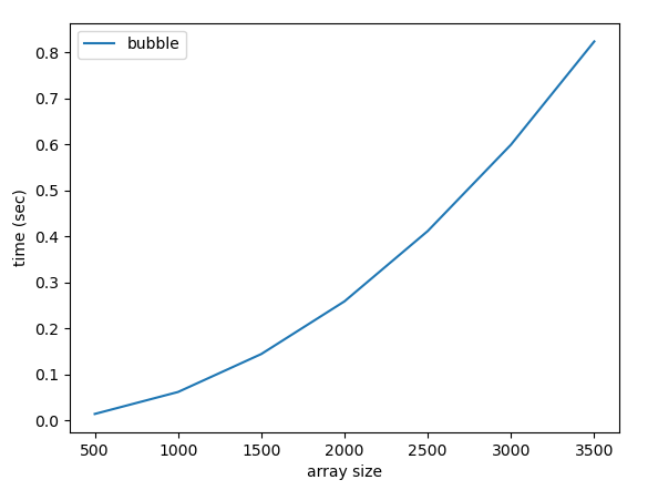
plt.show()The plot looks like this:
The quadratic shape is evident.
Our next sorting algorithm is selection sort. In a selection sort, we start by finding the smallest value in the array and exchanging it with the first element. We then find the second smallest value and exchange it with the second element, and so on. Here is an animation of selection sort in action.
Here's an implementation in Python:
def selection_sort(a):
    n = len(a)
    for i in range(n - 1):
        min_index = i
        min_val = a[i]
        for j in range(i + 1, n):
            if a[j] < min_val:
                min_val = a[j]
                min_index = j
        a[i], a[min_index] = a[min_index], a[i]
We can analyze selection sort's running time similarly to bubble sort. Just as in bubble sort, the total number of comparisons is
(N – 1) + (N – 2) + … + 2 + 1 = N(N – 1) / 2 = O(N2)
and the running time is O(N2) in the best and worst case. However, selection sort will usually outperform bubble sort by as much as a factor of 2 to 3. That's because it performs many fewer swaps as it rearranges the data.
Let's extend the plot above to include a selection sort. To do that, we'll modify our test() function so that it takes an extra argument f indicating a sorting function to run. This is a feature of Python that we haven't seen yet: a variable or parameter can actually hold a function. (We will explore this concept more in a future lecture.)
# f is a sorting function
def test(n, f):
    a = []
    for i in range(n):
        a.append(randrange(1000))

    start = time.time()
    f(a)
    return time.time() - start

def plot():
    xs = range(500, 4000, 500)
    bub = []  # bubble
    sel = []  # selection
    for n in xs:
        print(f'n = {n}')
        bub.append(test(n, bubble_sort))
        sel.append(test(n, selection_sort))

    plt.plot(xs, bub, label = 'bubble')
    plt.plot(xs, sel, label = 'selection')
    plt.legend()
    plt.show()
Here is the result:

We can see that selection sort is significantly faster than bubble sort, perhaps by a factor of 2 to 3 in this Python implementation. However, selection sort is still evidently quadratic.