Big-O notation is a way to describe how fast a function may grow. We'll use it very often in this course.
In these notes we'll first describe big-O notation purely mathematically. After that, we'll see how we can use it to describe the running time of a program or algorithm.
Here is a first, slightly informal definition of big-O notation. Suppose that f and g are functions. Informally, we say that f(n) = O(g(n)) if f is eventually bounded by some constant times g, or, equivalently, that f does not grow faster than g. (Recall that in the last lecture we said that f(n) grows faster than g(n) if the ratio f(n) / g(n) becomes arbitrarily large as n increases.)
For example, we may write that
2n + 3 = O(n)
3n2 + 2n + 5 = O(n2)
2n + n4 = O(2n)
Notice that we can generally describe a function in big-O notation by discarding all lower-order terms, plus any constant factor. For example, if we're given 3n2 + 2n + 5, we can discard the lower-order terms (2n and 5), plus the constant factor 3, and we're left with n2.
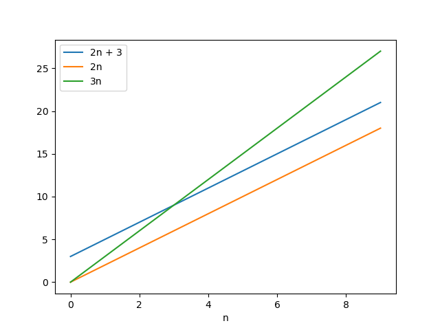
Now let's see how our informal definition applies to these statements. Consider the first of these statements: 2n + 3 = O(n). Here is a graph of f(n) = 2n + 3 plus a couple of other functions:
Notice that f(n) = 2n + 3 is not bounded by the function 2n, since it's always greater than 2n. However f is eventually bounded by the function 3n. Although 2n + 3 > 3n for small values of n, at a certain point (namely n = 3) 2n + 3 = 3n, and whenever n > 3 we have 2n + 3 < 3n. So 3n, which is a constant times n, is eventually an upper bound for f. For that reason, we can say that 2n + 3 = O(n).
As another example, consider the statement 3n2 + 2n + 5 = O(n2). Here's a graph of f(n) = 3n2 + 2n + 5, plus some other functions:
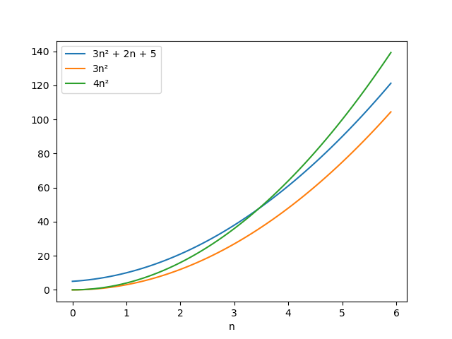
Again, notice that whenever n is greater than a certain value, then 3n2 + 2n + 5 is less than 4n2, i.e. a constant times n2. For this reason we can say that 3n2 + 2n + 5 = O(n2). (In fact the constant 4 is arbitrary; we could choose any value c > 3, and 3n2 + 2n + 5 would be eventually bounded by cn2.)
Now let's look at two more formal definitions. We may define big-O notation as follows:
1) f(n) = O(g(n)) if there exist constants c > 0, n0 > 0 such that for all n ≥ n0, f(n) ≤ c ⋅ g(n)
Alternatively, here is a definition using limits:
2) f(n) = O(g(n)) if lim n→∞ [ f(n) / g(n) ] = C for some 0 ≤ C < ∞
Let's formally prove that 2n + 3 = O(n). Let f(n) = 2n + 3 and g(n) = n. Using the first definition above, we need to choose the constants c and n0. Let c = 3, as in the first graph above. And let n0 = 3, since this is the value of n for which 2n + 3 = 3n. So now whenever n ≥ n0, we have 2n + n ≥ 2n + 3, so 3n ≥ 2n + 3, so f(n) ≤ c ⋅ g(n).
Alternatively, we can use the second definition. lim n→∞ [ f(n) / g(n) ] = lim n→∞ [ (2n + 3) / n ] = 2, which is less than ∞. That was easier!
Definitions (1) and (2) are almost equivalent, but not completely so due to a technicality: lim n→∞ [ f(n) / g(n) ] might not exist. For example, according to the first definition sin(n) = O(1) since we always have sin(n) ≤ 1, however we can't use the second definition to show this since lim n→∞ [ sin(n) / 1 ] is undefined. For this reason, definition (1) is the most general. Still, when the limit exists I generally find definition (2) easier to use.
We would like to consider how long our programs take to run as a function of their input size. For example, if a program sorts a list of numbers, the input size will be the length of the list. If a program simply takes an integer N as its input (such as program that tests whether N is prime), we will let the input size be N itself. We will express the running time as a big-O function of N. Sometimes this is called an asymptotic running time.
Now, in many programs there will be many different possible inputs of a given size. For example, consider a program that sorts a list of numbers. There are many different possible lists of numbers of a given length N, and some of these might be harder to sort than others (as we will see soon). Generally we will say that a program P runs in time O(f(N)) if P runs in that amount of time for all possible inputs of any size N. (If a program simply takes an integer N as input, then this is not a consideration since there is only possible input of size N, namely the integer N itself.)
In general in this course we will assume that numeric operations such as +, -, * and // run in constant time. Strictly speaking, that is not true since integers in Python can be arbitrarily large. However, this is a common assumption that will make our analysis easier. (Many languages such as C and C++ have fixed-size integers; in these languages, the running time of numeric operations is actually constant.)
As a first example, consider this code, which computes a certain function of an input number n:
n = int(input('Enter n: '))
sum = 0

for i in range(n):
    sum += i

    for j in range(n):
        sum += i * j

print('The answer is', sum)
Here the input size is n. This code will run quickly when n is small, but as n increases the running time will certainly increase. How can we quantify this?
Here is the same code again, with comments indicating how many times each line will run:
n = int(input('Enter n: '))

sum = 0                        # 1 time

for i in range(1, n + 1):      # n times
    sum += i                   # n times

    for j in range(1, n + 1):  # n * n times
        sum += i * j           # n * n times

print('The answer is', sum)
Suppose that the 5 commented statements above will run in times A, B, C, D, and E, where these letters are constants representing numbers of nanoseconds. Then the total running time is A + (B + C) n + (D + E) n2. This is O(n2), since we can discard the lower-order terms (A and (B + C)n) as well as the constant factor (D + E).
Coming back to our previous example, let's make a slight change to the code:
n = int(input('Enter n: '))

sum = 0

for i in range(1, n + 1):      # 1 .. n
    sum += i

    for j in range(1, i + 1):  # 1 .. i
        sum += i * j

print('The answer is', sum)
What is its running time now?
Once again the statement "sum = 0" will execute once, and the statements "for i" and "sum += i" will execute n times. The statements "for j" and "s += i * j" will execute 1 time on the first iteration of the outer loop (when i = 2), 2 times on the next iteration (when i = 2) and so on. The total number of times they will execute is
1 + 2 + … + n = n (n + 1) / 2 = n2 / 2 + n / 2 = O(n2)
Thus, the code's running time is still O(n2).
This example illustrates an important principle that we will see many times in the course, namely that
1 + 2 + 3 + … + N = O(N2)
Let's consider the running time of the algorithms on integers that we have already studied in this course.
In the first lecture we saw how to extract digits in any base. For example, consider this program to extract the digits of an integer in base 7:
n = int(input('Enter n: '))

while n > 0:
    d = n % 7
    print(d)
n = n // 7What is its asymptotic running time as a function of n, the given number?
The body of the 'while' loop runs in constant time, since we've assumed that arithmetic operations run in constant time. So we only need to consider how many times the loop will iterate.
The question, then, is this: given an integer n, how many digits will it have in base 7?
If the answer is not obvious, consider an example in base 10. Let n = 123,456,789. This number has 9 digits. Notice that
108 = 100,000,000 < n < 1,000,000,000 = 109
Taking logarithms, we see that
8 < log10 n < 9
So we see that the number of digits of n in base 10 is log10 n, rounded up to the next integer.
Then of course in base 7 the number of digits will be log7 n, rounded up to the next integer. The rounding adds a value less than 1 and does not affect the big-O running time: big O does not care about adding (or multiplying by) a constant. So we can ignore the rounding. And so the program runs in O(log7 n).
Now, when we write O(log n) normally we never write a base for the logarithm. That's because logarithms in two different bases differ by only a constant factor. For example, log7 n = log10 n ⋅ log7 10, and log7 10 is of course a constant. So we can simply say that this program runs in O(log n).
Now let's look at primality testing using trial division, which we saw in the last lecture:
from math import sqrt

n = int(input('Enter n: '))

prime = True
for i in range(2, int(sqrt(n)) + 1):
    if n % i == 0:
        prime = False
        break

if prime:
    print('n is prime')
else:
    print('not prime')
Let the input size be the number n.
Often we are interested in determining an algorithm's best-case and worst-case running times as a function of n. For some algorithms these times will be the same, and for others they will be different. The best-case running time is a lower bound on how long it might take the algorithm to run when n is large, and the worst-case running time is an upper bound.
In the best case in this program, N might be an even number. Then even if n is extremely large, the 'for' loop will exit immediately since n is divisible by 2. So this function runs in O(1) in the best case. In the worst case, N is a prime number, and the loop must iterate O(√N) times to establish its primality. So the program runs in O(√N) in the worst case.
Now, be wary of a mistake that I've sometimes seen first-year students make. Occasionally a student will say "This program's best-case running time is O(1) because the input size N might be small, in which case the program will exit immediately". That logic is incorrect. By that argument, pretty much every algorithm would run in O(1) in the best case! We may say that an algorithm runs in O(g(n)) in the best case only if the running time is O(g(n)) for some arbitrarily large inputs. In this example, even when N is very large it may be even and the loop may exit immediately, so the best-case time really is O(1).
(More formally, we may say that an algorithm runs in O(g(n)) in the best case if there exists some infinite set B of possible inputs such that (1) the values in B are of unbounded size, i.e. for every value s there is some element of B whose size is greater than s, and (2) the algorithm runs in time O(g(n)) on all inputs in B. In this example, B is the set of positive even integers.)
Next, let's revisit our integer factorization algorithm:
from math import sqrt

n = int(input('Enter n: '))

f = 2
s = ''
while f <= int(sqrt(n)):
    if n % f == 0:  # n is divisible by f
        s += f'{f} * '
        n = n // f
    else:
        f += 1

s += str(n)     # append the last factor
print(s)
In the worst case, n is prime, and the test 'if n % f == 0'
will execute √n – 1 times. Thus the worst-case running time is
O(√n).
Now suppose that n is a power of 2. Then the test
'if n % i == 0' will run log2 n – 1 times,
and the program will run in O(log2 n) = O(log n). So the
best-case running time is at most O(log n) (and is probably even
slightly less that that, though a precise analysis is beyond our
discussion today).
In the last lecture we studied Euclid’s algorithm for computing the greatest common divisor of two integers. We saw that at each step Euclid's algorithm replaces the integers a, b with the integers b, a mod b. So, for example,
gcd(252, 90)
=
gcd(90, 72)
= gcd(72, 18)
= gcd(18, 0)
= 18
We'd now like to consider the running time of Euclid's algorithm when computing gcd(a, b). We must first define the input size N. Assume that a > b, and let N = a.
Notice that for any integers a, b with a > b, we have
(a mod b) < a / 2
To see this, consider two cases. In case (1), suppose that b ≤ a / 2. Then (a mod b) ≤ b – 1, since any value mod b must be less than b. So a mod b < a / 2. Or, in case (2), we have b > a / 2. Then a div b = 1, so (a mod b) = a – b < a – a / 2 = a / 2.
Now suppose that we call gcd(a, b), and consider the values at each iteration:
iteration 1: a, b
iteration 2: b, a mod b
iteration 3: a mod b, b mod (a mod b)
...
In the first two iterations the first argument has dropped from a to (a mod b), which is less than a / 2. So after every two iterations of the algorithm, the first argument will be reduced by at least a factor of 2. This shows that the algorithm cannot iterate more than 2 log2(a) times before a reaches 1, at which point the algorithm terminates. And so the algorithm runs in time O(2 log a) = O(log a) = O(log N) in the worst case, since N = a.
We've seen in previous lectures that we can determine whether an integer n is prime using trial division, in which we attempt to divide n by successive integers. Because we must only check integers up to √n, this primality test runs in time O(√n).
Sometimes we may wish to generate all prime numbers up to some limit N. If we use trial division on each candidate, then we can find all these primes in time O(N √N). But there is a faster way, using a classic algorithm called the sieve of Eratosthenes.
It's not hard to carry out the sieve of Eratosthenes using pencil and paper. It works as follows. First we write down all the integers from 2 to N in succession. We then mark the first integer on the left (2) as prime. Then we cross out all the multiples of 2. Now we mark the next unmarked integer on the left (3) as prime and cross out all the multiples of 3. We can now mark the next unmarked integer (5) as prime and cross out its multiples, and so on.
Here is the result of using the sieve of Eratosthenes to generate all primes between 2 and 30:
2
3 4
5 6
7 8
9 10
11 12
13 14
15 16
17 18
19 20
21 22
23 24
25 26
27 28
29 30
We can easily implement the sieve of Eratosthenes in Python. Here's a program that generates and prints all prime numbers up to a given number n:
n = int(input('Enter n: '))

prime = (n + 1) * [ True ]    # initially assume all are prime

prime[0] = prime[1] = False   # 0 and 1 are not prime

for i in range(2, n + 1):   # 2 .. n
    if prime[i]:
        # cross off multiples of i
        for j in range(2 * i, n + 1, i):
            prime[j] = False

for i in range(2, n + 1):    # 2 .. n
    if prime[i]:
        print(i)
How long does the sieve of Eratosthenes take to run?
The inner loop, in which we set prime[j]
= False, runs
N / 2 times when we cross out all the multiples of 2, then N / 3
times when we cross out multiples of 3, and so on. So its total
number of iterations will be close to
N(1/2 + 1/3 + 1/5 + ... + 1/N)
The series of reciprocals of primes
1/2 + 1/3 + 1/5 + 1/7 + 1/11 + 1/13 + ...
is called the prime harmonic series. How can we approximate its sum through a given element 1/p?
Euler was the first to show that the prime harmonic series diverges: its sum grows to infinity, through extremely slowly. Its partial sum through 1/p is actually close to ln (ln n). (Recall that the natural logarithm ln(n) is loge(n).) And so the running time of the Sieve of Eratosthenes is
O(N(1/2 + 1/3 + 1/5 + ... + 1/N)) = O(N log log N)
This is very close to O(N). (As always, we are assuming that arithmetic operations take constant time.)
The sieve of Eratosthenes is already very efficient, but we can optimize it slightly. When we cross off multiples of i, actually we can start at the value i2, because any smaller multiples of i will already have been eliminated when we considered smaller values of i. That in turn means that we only need to consider values of i up to √n.
Here is an optimized version of the code above, with changes in red:
prime = (n + 1) * [ True ] # initially assume all are prime
prime[0] = prime[1] = False # 0 and 1 are not prime
for i in range(2, int(sqrt(n)) + 1): # 2 .. sqrt(n)
if prime[i]:
# cross off multiples of i
for j in range(i * i, n + 1, i):
prime[j]
=
False