Week 13: Notes

stable sorting

In earlier weeks we saw that we can modify any sorting algorithm so that it sorts using a key function, which maps each element to a key used for sorting. For example, here's an implementation of insertion sort with a key function:

# f maps a value to a sorting key
def insertion_sort_by(a, f):
    n = len(a)
    for i in range(n):
        k = a[i]
        j = i - 1
        while j >= 0 and f(a[j]) > f(k):
            a[j + 1] = a[j]
            j -= 1
        a[j + 1] = k

Suppose that we would like to sort this array of strings by length:

>>> a = ['town', 'grape', 'prague', 'two', 'night', 'day', 'one', 'lift']

Then the key function maps each string to its length. Let's sort the array using the insertion sort function above:

>>> insertion_sort_by(a, len)
>>> a
['two', 'day', 'one', 'town', 'lift', 'grape', 'night', 'prague']

We see that the sorted array contains all strings of length 3, then strings of length 4, and so on. Furthermore, for any value k, the strings of length k appear in the same order as in the original array. That is guaranteed because insertion sort is stable. A stable sorting algorithm preserves the order of values with the same key.

Some sorting algorthms are naturally stable, and others are not. For example, bubblesort is stable because it will never swap two values with the same key, so their order will be preserved throughout the sort. Of the other algorithms that we've seen in this course, insertion sort and merge sort are stable; selection sort, quicksort and heap sort are not. You may want to think about why.

An interesting property of a stable sorting algorithm is that if you first sort values with a key function f₁, then sort them again by a key function f₂, the resulting array will be sorted primarly by f₂, with f₁ used to break ties for values that f₂ maps to the same key. That means that if x will precede y in the array if f₂(x) < f₂(y), or if f₂(x) = f₂(y) and f₁(x) < f₁(y). To put it differently, this is like sorting by a key function f(x) that generates the pair (f₂(x), f₁(x)), where pairs are compared lexicographically.

For example, suppose that we have a list of students and their ages in a file called "students":

Liam 20
Amelia 19
Henry 21
Ava 18
William 19
Emma 19
Lucas 22
Olivia 21
Mia 20
Luna 20
James 22
Oliver 18

Let's load this data into a list of Student objects:

from dataclasses import dataclass

@dataclass
class Student:
    name: str
    age: int

students = []
with open('students') as f:
    for line in f:
        name, age = line.split()
        students.append(Student(name, int(age)))

Let's first sort the students by name, then by age. We'll use insertion sort, which is stable:

>>> insertion_sort_by(students, lambda s: s.name)
>>> insertion_sort_by(students, lambda s: s.age)

Now let's look at the resulting list:

>>> from pprint import pprint
>>> pprint(students)
[Student(name='Ava', age=18),
 Student(name='Oliver', age=18),
 Student(name='Amelia', age=19),
 Student(name='Emma', age=19),
 Student(name='William', age=19),
 Student(name='Liam', age=20),
 Student(name='Luna', age=20),
 Student(name='Mia', age=20),
 Student(name='Henry', age=21),
 Student(name='Olivia', age=21),
 Student(name='James', age=22),
 Student(name='Lucas', age=22)]

We see that the students are sorted primarily by age and secondarily by name. For example, the three students with age 19 appear in alphabetical order (Amelia, Emma, William). If we had used a non-stable sorting algorithm, we'd end up with a list sorted by age, but the alphabetical order of students with the same age might not be preserved.

counting sort

In a lecture a few weeks ago, we saw that no comparison-based sorting algorithm can run in better than O(N log N) time in the worst case.

However there do exist some sorting algorithms that can run in linear time! These algorithms are not comparison-based, and so they are not as general as the other sorting algorithms we've studied in this course. In other words, they will work only on certain types of input data.

As a first example, consider sorting an array of booleans such as

[True, False, False, True, False, True, True, False, True]

We consider False to be less than True, so we want to produce an array such as

[False, False, False, False, True, True, True, True, True]

We could perform this sort using any of the sorting algorithms we've already seen. However, another approach is simple and more efficient. We will first iterate over the array and count the number of elements that are True. Suppose that the input array contains N booleans, and we find that (t) of them are True. Then (N - t) must be False. So once we know (t), we can make another pass over the array, and fill in the first (N - t) values with False and the remaining (t) values with True. The entire algorithm will run in O(N).

We may generalize this idea into an algorithm called counting sort. In its simplest form, counting sort works on an input array of integers in the range 0 ≤ i < k for some fixed integer k. The algorithm traverses the input array and builds a table that maps each integer i (0 ≤ i < k) to a value count[i] indicating how many times it occurred in the input. After that, it makes a second pass over the input array, writing each integer i exactly count[i] times as it does so.

For example, suppose that k = 5 and the input array is

2 4 0 1 2 1 4 4 2 0

The table of counts will look like this:

• count[0] = 2

• count[1] = 2

• count[2] = 3

• count[3] = 0

• count[4] = 3

So during the second pass the algorithm will write two 0s, two 1s, three 2s and so on. The result will be

0 0 1 1 2 2 2 4 4 4

Here is an implementation:

# Sort the array a, which contains integers in the range 0 .. (k - 1).
def counting_sort(a, k):
    count = k * [0]

    for x in a:
        count[x] += 1

    j = 0
    for i in range(k):
        for _ in range(count[i]):
            a[j] = i
            j += 1  

Let's consider the running time of this function, where N is the length of the input array a. Allocating the array 'count' will take time O(k). The first 'for' loop runs in O(N), since it examines each input value once. The second, nested 'for' loop examines all values in the 'count' array, which takes O(k). It also runs the statements 'a[j] = i' and 'j += 1' a total of N times, which takes O(N). The total running time is O(k + N). We consider k to be a constant, so this is O(N).

counting sort with a key

Let's modify the counting sort algorithm so that it uses a key function. The input to the algorithm will be an array a, plus a key function f that maps each element of a to an integer in the range 0 .. (k – 1) for some fixed integer k. We'd like to produce an array containing all the values in a, sorted by key. As an additional requirement, we would like this sort to be stable.

We can allocate an array of k buckets, each intially containing the empty list. We'll then iterate over the input array; for each value x, we append x to the list in bucket f(x). After than, we need only concatenate the lists in all the buckets. Here is an implementation in Python:

# f maps each value to a value in the range 0 .. (k - 1)
def counting_sort_by(a, f, k):
    vals = [[] for _ in range(k)]
    for x in a:
        vals[f(x)].append(x)
    
    i = 0
    for vs in vals:
        for v in vs:
            a[i] = v
            i += 1

Assume that the input array a has N elements, and that the key function f runs in constant time. How long will this function take to run, as a function of N? Allocating the buckets takes O(k). The first 'for' loop above will run in O(N) since Python's append() method runs in O(1) on average. The second 'for' loop will run in O(k + N), since it examines all k buckets and appends every element exactly once. The total running time is O(k + N), which is O(N) since k is a constant. The sort is stable, since each bucket contains values in the same order in which they appeared in the original array.

performance of counting sort

We know that counting sort runs in linear time, but how does its performance actually compare with quicksort, which is the fastest algorithm we've seen previously? Let's make a plot showing the time that these algorithms take to sort an array of N numbers in the range 0 ≤ i < 1000:

import time
import matplotlib.pyplot as plt

def quicksort(a):
   ...

def counting_sort(a, k):
   ...

# f is a sorting function
def test(n, f):
    a = []
    for i in range(n):
        a.append(randrange(1000))

    start = time.time()
    f(a)
    return time.time() - start

def plot():
    xs = range(5000, 100_000, 5000)
    qui = []
    cou = []
    for n in xs:
        print(f'n = {n}')
        qui.append(test(n, quicksort))
        cou.append(test(n, lambda a: counting_sort(a, 1000)))

    plt.plot(xs, qui, label = 'quicksort')
    plt.plot(xs, cou, label = 'counting_sort(1000)')
    plt.legend()
    plt.show()

Here is the result:

We see that counting sort is far faster than quicksort when sorting numbers in this range.

Now let's modify the code above to sort numbers in the range 0 ≤ i < 1,000,000. Here is the resulting plot:

We see that the cost of allocating and traversing an array with 1,000,000 elements is significant, and quicksort outperforms counting sort when sorting less than about 50,000 numbers in this range.

radix sort

When we use a counting sort to sort integers in the range 0 ≤ i < k, the sort will allocate an array with k elements. As we've seen, that is reasonable as long as k is small. But what if M is a large number such as 1,000,000,000 or 1,000,000,000,000, a counting sort is not practical.

Radix sort is another algorithm that can sort an array of integers up to a fixed value k. Like counting sort, it runs in time O(N), where there are N integers in the input array. However it will generally use far less memory than a counting sort, and is practical even for large values of k such as k = 1,000,000,000,000.

Radix sort works by performing a series of passes. In each pass, it uses a stable counting sort to sort the input numbers by a certain digit. In the first pass, this is the last digit of the input numbers. In the second pass, it is the second-to-last digit, and so on. After all passes are complete, the array will be sorted.

For example, consider the operation of radix sort on these numbers:

503 223 652 251 521 602

In the first pass, we sort by the last digit. The sort is stable, so if numbers have the same digit, their order will be preserved:

251 521 652 602 503 223

Next we sort by the middle digit:

602 503 521 223 251 652

Finally, we sort by the first digit:

223 251 503 521 602 652

The sort is complete, and the numbers are in order.

Why does radix sort work? After the first pass, the numbers are sorted by their last digit. In the second pass, we sort numbers by the second-to-last digit. Ties will be resolved using the previous ordering (since counting sort is stable), which is by the last digit, so after the second pass all numbers will be sorted by their last two digits. After another pass, the numbers will be sorted by their last three digits, and so on.

Here is an implementation in Python:

# Sort an array a of numbers that have up to k decimal digits.
def radix_sort(a, d):
    p = 1
    for _ in range(d):
        a = counting_sort_by(a, 10, lambda x: (x // p) % 10)
        p *= 10
    return a

If we consider the number of digits d to be a constant, then the algorithm makes a constant number of passes. Each pass runs in O(N), so the total running time is d · O(N) = O(N).

Let's use our plotting code to compare the time of radix sort versus quicksort, for sorting values in the range 0 ≤ i < 1,000,000,000. These values may have up to 9 digits, so we'll pass d = 9 to the radix_sort function above. Here is the result:

We see that our implementation of radix sort performs about as well as quicksort.

However, we can do better. The code above uses base 10, but of course the base is arbitrary. Let's generalize our radix sort function so that we can specify the base:

# Sort numbers with up to d digits in the given base.
def radix_sort(a, base, d):
    p = 1
    for _ in range(d):
        counting_sort_by(a, base, lambda x: (x // p) % base )
        p *= base

Let's once again sort a set of numbers in the range 0 ≤ i < 1,000,000,000, but using a larger base. We'll choose base 1000, which will consider each number as a series of digits in base 1000. For example, consider the number 638970283. This number has 9 digits in base 10, but only 3 digits in base 1000. Those digits are [638], [970] and [283]. That is because

638970283 = 638 ⋅ 1000² + 970 ⋅ 1000 + 283 ⋅ 1

Any number with up to 9 decimal digits will have up to 3 digits in base 1000, so we can sort these numbers by calling radix_sort(a, 1000, 3). Let's do that, and plot the resulting performance:

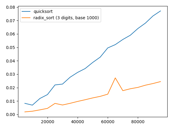
We see that radix sort with base 1000 significantly outperforms quicksort when sorting numbers in this range.