
In Python, you may use if
and else inside an expression;
this is called a conditional expression.
For example, consider this code:
if x > 100:
    print('x is big')
else:
    print('x is not so big')
We may rewrite it using a conditional expression:
print('x is ' + ('big' if x > 100 else 'not so big'))As another example, here is a function that takes two integers and returns whichever has the greater magnitude (i.e. absolute value):
def greater(i, j):
   if abs(i) >= abs(j):
       return i
   else:
       return j
We can rewrite it using a conditional expression:
def greater(i, j):
    return i if abs(i) >= abs(j) else j
(If you already know C or another C-like language, you may notice this feature's resemblance to the ternary operator (? :) in those languages.)
Python allows a 'while' or 'for' statement to contain an 'else' clause, which will execute if the loop does not exit via a 'break' statement. This is an unusual feature among programming languages, but can sometimes be convenient. For example, consider a program that checks whether a number is prime:
n = int(input())

i = 2
prime = True
while i * i <= n:
    if n % i == 0:
        prime = False
        break
    i += 1

if prime:
    print('prime')
else:
    print('composite')
We may rewrite this program without the boolean variable 'prime', by adding an 'else' clause to the 'while' statement:
n = int(input())

i = 2
while i * i <= n:
    if n % i == 0:
        print('prime')
        break
    i += 1
else:
print('composite')A list may contain any type of elements, including tuples or sublists:
>>> l = [(2, 3), (10, 20), (5, 6)]

>>> m = [[2, 4, 6], [5, 7, 9], [1, 3, 5]]
We can use nested lists to solve many two-dimensional problems. In particular, a list of lists is a natural way to represent a matrix in Python. Consider this matrix with dimension 3 x 3:
5  11  12
2   8   7
14  2   6
If we want to store it in Python as a list of lists, we have two choices. We could store the matrix in row-major order, in which each sublist holds a row of the matrix:
m = [ [5, 11, 12], [2, 8, 7], [14, 2, 6] ]
Or we can use column-major order, in which each sublist is a matrix column:
m = [ [5, 2, 14], [11, 8, 2], [12, 7, 6] ]
The choice is arbitrary. However, usually by convention we will use row-major order. With this ordering, we can use the syntax m[i][j] to access the matrix element at row i, column j.
Let's write a function that takes an integer n and returns an identity matrix of size n x n. Recall that an identity matrix has ones along the main diagonal, and zeroes everywhere else. For example:
1 0 0 0
0 1 0 0
0 0 1 0
0 0 0 1
In our function, we will first create an n x n matrix of zeroes, then fill in the diagonal with ones.
Recall that we can use the * operator to create a list with repeated elements:
>>> 10 * [0]
[0, 0, 0, 0, 0, 0, 0, 0, 0, 0]
So you might think that you can create a matrix of zeroes by using that operator twice:
# WRONG – DON'T DO THIS
>>> m = 4 * [4 * [0]]
>>> m
[[0, 0, 0, 0], [0, 0, 0, 0], [0, 0, 0, 0], [0, 0, 0, 0]]
As the comment above indicates, this is a bad idea. The problem with this approach is that the sublists will be shared, i.e. all four sublists are actually the same list! To see this, let's try setting the upper-left element to 7, then look at the resulting list:
>>> m[0][0] = 7
>>> m
[[7, 0, 0, 0], [7, 0, 0, 0], [7, 0, 0, 0], [7, 0, 0, 0]]
That's evidently wrong.
Instead, we can create a matrix of zeroes using a loop. In each iteration, we will create a row of zeroes and add it to our matrix. Here is the complete function to create an identity matrix:
# Return the identity matrix of dimensions n x n.
def identity(n):
    # create matrix of zeroes
    m = []
    for i in range(n):
        m.append(n * [0])

    # fill in diagonal
    for i in range(n):
        m[i][i] = 1

return mA recursive function calls itself. Recursion is a powerful technique that can help us solve many problems.
When we solve a problem recursively, we express its solution in terms of smaller instances of the same problem. The idea of recursion is fundamental in mathematics as well as in computer science.
As a first example, consider this function that computes n! for any positive integer n. (Recall that n! = n · (n – 1) · … · 3 · 2 · 1.) It uses a loop, so this is an iterative function:
def factorial(n):
    p = 1

    for i in range(1, n + 1):
        p *= i

    return p
We can rewrite this function using recursion. Now it calls itself:
def factorial(n):
    if n == 0:
        return 1     # 0! is 1

    return n * factorial(n - 1)
Whenever we write a recursive function, there is a base case and a recursive case.
The base case is an instance that we can solve immediately. In the function above, the base case is when n == 0. A recursive function must always have a base case – otherwise it would loop forever since it would always call itself!
In the recursive case, a function calls itself, passing it a smaller instance of the given problem. Then it uses the return value from the recursive call to construct a value that it itself can return.
In the recursive case in this example, we
recursively call factorial(n -
1). We then multiply its return value by
n, and return that value. That works because
n! = n · (n – 1)! whenever n ≥ 1
(In fact, we may treat this equation as a recursive definition of the factorial function, mathematically speaking.)
How does this function work, exactly? Suppose that we call factorial(3). It will call factorial(2), which calls factorial(1), which calls factorial(0). The call stack in memory now looks like this:
factorial(3)
→ factorial(2)
  → factorial(1)
    → factorial(0)
Now
factorial(0) returns 1 to its caller factorial(1).
factorial(1) takes this value 1, multiplies it by n = 1 and returns 1 to factorial(2).
factorial(2) takes this value 1, multiplies it by n = 2 and returns 2 to factorial(3).
factorial(3) takes this value 2, multiplies it by n = 3 and returns 6.
We see that given any n, the function returns the sum 1 * 2 * 3 * … * n = n!.
We have seen that we can write the factorial function either iteratively (i.e. using loops) or recursively. In theory, any function can be written either iteratively or recursively. We will see that for some problems a recursive solution is easy and an iterative solution would be quite difficult. Conversely, some problems are easier to solve iteratively. Python lets us write functions either way.
Here is some general advice for writing a recursive function. First look for base case(s) where the function can return immediately. Now you need to write the recursive case, where the function calls itself. At this point you may wish to pretend that the function "already works". Write the recursive call and believe that it will return a correct solution to a subproblem, i.e. a smaller instance of the problem. Now you must somehow transform that subproblem solution into a solution to the entire problem, and return it. This is really the key step: understanding the recursive structure of the problem, i.e. how a solution can be derived from a subproblem solution.
Here's another example. Consider this implementation of Euclid's algorithm that we saw in Intro to Algorithms:
# gcd, iteratively
def gcd(a, b):
    while b > 0:
        a, b = b, a % b

    return a
We can rewrite this function using recursion:
# gcd, recursively
def gcd(a, b):
    if b == 0:
        return a

    return gcd(b, a % b)
Broadly speaking, we will see that
"easy" recursive functions such as gcd
call themselves only once, and it
would be straightforward to write them either iteratively or
recursively. Soon
we will see recursive
functions that call themselves two or more times. Those functions
will let us solve more difficult tasks that we could not easily solve
iteratively.
Here is another example of a recursive function:
def hi(x):
    if x == 0:
        print('hi')
        return

    print('start', x)
    hi(x - 1)
    print('done', x)
If we call hi(3), the output will be
start 3
start 2
start 1
hi
done 1
done 2
done 3
Be sure you understand why the lines beginning with 'done' are printed. hi(3) calls hi(2), which calls hi(1), which calls hi(0). At the moment that hi(0) runs, all of these function invocations are active and are present in memory on the call stack:
hi(3)
→ hi(2)
  → hi(1)
    → hi(0)
Each function invocation has its own value of the parameter x. (If this procedure had local variables, each invocation would have a separate set of variable values as well.)
When hi(0) returns, it does not exit from this entire set of calls. It returns to its caller, i.e. hi(1). hi(1) now resumes execution and writes 'done 1'. Then it returns to hi(2), which writes 'done 2', and so on.
All the recursive examples above were functions that we could easily write either recursively or iteratively. Now let's start to look at functions that would not be so straightforward to write in an iterative fashion, and for which recursion will be especially helpful.
As a first example, consider the directory structure of a typical filesystem. The root directory has subdirectories, which in turn have their own subdirectories, and so on. In other words, the structure is itself recursive.
Let's write a recursive function that takes the name of a directory, and prints out the paths of all files in the directory and its subdirectories, recursively. To write this function, we'll need to use functions in the os module that can ask for a list of all items in a directory, and can determine which of those items are files and which are subdirectories.
Here is the code:
import os

def enum(dir):
    for name in os.listdir(dir):
        path = os.path.join(dir, name)
        if os.path.isdir(path):
            enum(path)
        else:
            print(path)
When I run this function to enumerate all files in my Desktop directory, the output begins like this:
>>> list('/home/adam/Desktop')
/home/adam/Desktop/tutorials
/home/adam/Desktop/lecture/dirs.py
/home/adam/Desktop/lecture/recurse.py
/home/adam/Desktop/lecture/matrix.py
/home/adam/Desktop/lecture/diag.py
/home/adam/Desktop/lecture/matrix
/home/adam/Desktop/lecture/out
/home/adam/Desktop/lecture/picture.py
/home/adam/Desktop/lecture/fib.py
/home/adam/Desktop/lecture/prime.py
/home/adam/Desktop/apartments
/home/adam/Desktop/accounts.txt
/home/adam/Desktop/tutorial/missing.py
/home/adam/Desktop/tutorial/sample_in
…
Notice that there is no explicit base case written in the code above. The base case in this function occurs when a directory contains no subdirectories, in which case the function will not recurse.
Python
includes a module turtle
that
lets you draw simple graphics easily. In turtle graphics, you give
commands to a 'turtle' that always has an x-y position plus a current
heading, i.e. a direction that it is facing. When the turtle moves,
it draws a line if the virtual 'pen' is currently down. You can also
lift up the pen, in which case the turtle will move without drawing.
I've listed various functions from the turtle module on my Python quick reference page.
In Python's turtle graphics, the turtle begins at the origin (0, 0), which by default is at the center of the window. X coordinates increase to the right, and Y coordinates increase upward. (This is different from the usual convention in computer graphics, in which Y coordinates increase downward). If you prefer a different coordinate system, you can set one by calling the setworldcoordinates() function.
For example, here's a simple program to draw a 9-pointed star:
from turtle import *

for i in range(9):
    forward(200)
    left(160)

done()
The output looks like this:
Here's a program that draws 100 random lines. Each line connects two random points, each of which has an X-coordinate and Y-coordinate in the range from -200 to 200:
from random import randint
from turtle import *

for i in range(100):
    penup()
    goto(randint(-200, 200), randint(-200, 200))
    pendown()
    goto(randint(-200, 200), randint(-200, 200))

done()
The output looks like this:

Let's use recursion to draw a tree with turtle graphics. We can use a single recursive function to draw the entire tree and also to draw individual branches, since each branch will be similar to the tree as a whole. (A geometric figure that is self-similar in this way is sometimes said to be fractal.)
Here's a first attempt at the program:
from turtle import *

def draw(x, y, angle, length):
    if length < 10:
        return

    penup()
    goto(x, y)

    pendown()
    setheading(angle)
    forward(length)

    xpos, ypos = pos()
    draw(xpos, ypos, angle - 25, length * 0.75)
    draw(xpos, ypos, angle + 25, length * 0.75)

draw(0, -200, 90, 100)
done()
The recursive function draw() takes a position (x, y) at which to start drawing, as well as an angle and length for the first branch. It draws that branch, then calls itself twice recursively to draw the left and right subbranches, which are offset at angles of -25 and 25 degrees. On each recursive call, the function decreases the length by 25%. If the length is less than 10, the function returns without drawing anything; this is the base case.
The output looks like this:

The recursive structure of the tree is evident.
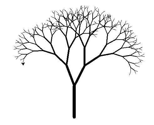
Let's modify the program so that it draws each branch with a thickness proportional to its length. Let's also add some randomness to the angles at which subbranches are offset, and also to the decrease in branch size:
from random import *
from turtle import *

def draw(x, y, angle, length):
    if length < 10:
        return

    penup()
    goto(x, y)

    pendown()
    setheading(angle)
    width(0.1 * length)
    forward(length)

    xpos, ypos = pos()
    draw(xpos, ypos, angle - uniform(20, 30), length * uniform(0.7, 0.8))
    draw(xpos, ypos, angle + uniform(20, 30), length * uniform(0.7, 0.8))

draw(0, -200, 90, 100)
done()
Now the output looks more like a real tree:
Generally speaking, there is a close relationship between recursion and trees. We will see many times both in the programming and algorithms classes that recursion explores a tree, which can be a data structure with a tree-like shape, or even a tree of possible solutions to some problem that we wish to solve. So recursion will be very helpful for us in the weeks ahead.