Week 6: Notes

recurrences

We have already studied how to analyze the running time of iterative functions, i.e. functions that use loops. We'd now like to do the same for recursive functions.

To analyze any recursive function's running time, we perform two steps. First, we write a recurrence, which is an equation that expresses the function's running time recursively, i.e. in terms of itself. Second, we solve the recurrence mathematically.

For example, consider this simple recursive function:

def fun1(n):
    if n == 0:
        return 0

    return n * n + fun1(n - 1)

The function computes the sum 1² + 2² + … + n², using recursion to perform its task.

Let's write down a recurrence that expresses this function's running time. Let T(N) be the time to run fun1(N). The function performs a constant amount of work outside the recursive call (since we generally assume that arithmetic operations run in constant time). When it calls itself recursively, n decreases by 1. And so we have the equations

T(0) = O(1)

T(N) = T(N - 1) + O(1)

Now we'd like to solve the recurrence. We can do so by expanding it algebraically. O(1) is some constant C. We have

T(N) = C + T(N - 1)
= C + C + T(N – 2)
= …
= C + C + ... + C
= N · C
= O(N)

The function runs in linear time. That's not a surprise, since an iterative loop to sum these numbers would also run in O(N).

When we write recurrences from now on, we will generally not bother to write a base case 'T(0) = O(1)', and will only write the recursive case, e.g. 'T(N) = T(N - 1) + O(1)'.

Now consider this function:

def fun2(n):
    if n == 0:
        return 0
    
    s = 0
    for i in range(n):
        s += n * i

    return s + fun2(n – 1)

The 'for' loop will run in O(N), so the running time will follow this recurrence:

T(N) = T(N – 1) + O(N)

We can expand this algebraically. O(N) is CN for some constant C, so we have

T(N) = CN + T(N – 1)
= CN + C(N – 1) + T(N – 2)
= CN + C(N – 1) + C(N - 2) + T(N - 3)
= …
= C(N + (N – 1) + … + 1)
= C(O(N²))
= O(N²)

As another example, consider this recursive function that computes the binary representation of an integer:

def fun3(n):
    if n == 0:
        return ''
    
    d = n % 2
    return fun3(n // 2) + str(d)

The work that the function does outside the recursive calls takes constant time, i.e. O(1). The function calls itself recursively at most once. When it calls itself, it passes the argument (n // 2). So we have

T(N) = T(N / 2) + O(1)

To solve this, let's again observe that O(1) is some constant C. We can write

T(N) = C + T(N / 2)
= C + C + T(N / 4)
= …
= C + C + ... + C (log₂(N) times)
= C log₂(N)
= O(log N)

Finally, consider this function:

def fun4(n):
    if n == 0:
        return 0
    
    s = 0
    for i in range(n):
        s += i * i
        
    return s + fun4(n // 2)

The running time follows this recurrence:

T(N) = T(N / 2) + O(N)

Let O(N) = CN. Then we have

T(N) = CN + T(N / 2)
= CN + C(N / 2) + T(N / 4)
= CN + C(N / 2) + C(N / 4) + T(N / 8)
…
= C(N + N / 2 + N / 4 + …)
= C(2N)
= O(N)

These recurrences were relatively easy to solve, since they arose from recursive functions that call themselves at most once. When we study recursive functions that call themselves twice or more, we will see recurrences that are not quite as easy.

merge sort, continued

In the last lecture we learned about the merge sort algorithm. Let's review the merge sort code that we saw in that lecture:

# Merge sorted arrays a and b into c, given that
# len(a) + len(b) = len(c).
def merge(a, b, c):
    i = j = 0     # index into a, b
    
    for k in range(len(c)):
        if j == len(b):      # no more elements available from b
            c[k] = a[i]      # so we take a[i]
            i += 1
        elif i == len(a):    # no more elements available from a
            c[k] = b[j]      # so we take b[j]
            j += 1
        elif a[i] < b[j]:
            c[k] = a[i]      # take a[i]
            i += 1
        else:
            c[k] = b[j]      # take b[j]
            j += 1

def merge_sort(a):
    if len(a) < 2:
        return
        
    mid = len(a) // 2
    
    left = a[:mid]      # copy of left half of array
    right = a[mid:]     # copy of right half
    
    merge_sort(left)
    merge_sort(right)
    
    merge(left, right, a)

We also performed a performance experiment in which we saw that merge sort was much faster than any of the quadratic sorting algorithms (bubble sort, selection sort, insertion sort) that we saw previously.

What is the actual big-O running time of merge sort? In the code above, the helper function merge runs in time O(N), where N is the length of the array c. The array slice operations a[:mid] and a[mid:] also take O(N). So if T(N) is the time to run merge_sort on an array with N elements, then we have

T(N) = 2 T(N / 2) + O(N)

We have not seen this recurrence before. Let's expand it algebraically. Let O(N) = CN for some constant C. We have

T(N) = CN + 2 T(N / 2)
= CN + 2 ( C (N / 2) + 2 T(N / 4))
= CN + CN + 4 T(N / 4)
= CN + CN + 4 ( C (N / 4) + 2 T(N / 8))
= CN + CN + CN + 8 T(N / 8)
= …
= CN + CN + … + CN + N T(1)
= (log₂ N) CN + N T(1)

T(N) = O(N log N)

Above, the term (log₂ N) appears because we must perform (log₂ N) divisions by 2 to reach the value 1.

For large N, O(N log N) is much faster than O(N²), so mergesort will be far faster than insertion sort or bubble sort. For example, suppose that we want to sort 1,000,000,000 numbers. And suppose (somewhat optimistically) that we can perform 1,000,000,000 operations per second. An insertion sort might take roughly N² = 1,000,000,000 * 1,000,000,000 operations, which will take 1,000,000,000 seconds, or about 32 years. A merge sort might take roughly N log N ≈ 30,000,000,000 operations, which will take 30 seconds. This is a dramatic difference!

We've seen that merge sort is quite efficient. However, one potential weakness of merge sort is that it will not run in place: it requires extra memory beyond that of the array that we wish to sort. That's because the merge step won't run in place: it requires us to merge two arrays into an array that is held in a different region of memory. So any implementation of merge sort must make a second copy of data at some point. (Ours does so in the lines 'left = a[:mid]' and 'right = a[mid:]', since an array slice in Python creates a copy of a range of elements.)

Quicksort

Quicksort is another sorting algorithm. It is efficient (typically significantly faster than mergesort) and is commonly used.

Quicksort sorts values in an array in place - unlike mergesort, which needs to use extra memory to perform merges. Given a range a[lo:hi] of values to sort in an array a, quicksort first arranges the elements in the range into two non-empty partitions a[lo:k] and a[k:hi] for some integer k. It does this in such a way that every element in the first partition (a[lo:k]) is less than or equal to every element in the second partition (a[k:hi]). After partitioning, quicksort recursively calls itself on each of the two partitions.

The high-level structure of quicksort is similar to mergesort: both algorithms divide the array in two and call themselves recursively on both halves. With quicksort, however, there is no more work to do after these recursive calls. Sorting both partitions completes the work of sorting the array that contains them. Another difference is that merge sort always divides the array into two equal-sized pieces, but in quicksort the two partitions are generally not the same size, and sometimes one may be much larger than the other.

Two different partitioning algorithms are in common use. In this course we will use Hoare partitioning, which works as follows. To partition a range of an array, we first choose some element in the range to use as the pivot. The pivot has some value p. Once the partition is complete, all elements in the first partition will have values less than or equal to p, and elements in the second partition will have values greater than or equal to p.

To partition the elements, we first define integer variables i and j representing array indexes. Initially i is positioned at the left end of the array and j is positioned at the right. We move i rightward, looking for a value that is greater than or equal to v (i.e. it can go into the second partition). And we move j leftward, looking for a value that is less than or equal to v. Once we have found these values, we swap a[i] and a[j]. After the swap, a[i] and a[j] now hold acceptable values for the left and right partitions, respectively. Now we continue the process, moving i to the right and j to the left. Eventually i and j meet. The point where they meet is the division point between the partitions, i.e. is the index k mentioned above.

Note that the pivot element itself may move to a different position during the partitioning process. There is nothing wrong with that. The pivot really just serves as an arbitrary value to use for separating the partitions.

For example, consider a partition operation on this array:

The array has n = 8 elements. Suppose that we choose 3 as our pivot. We begin by setting i = 0 and j = 7. a[0] = 6, which is greater than the pivot value 3. We move j leftward, looking for a value that is less than or equal to 3. We soon find a[6] = 2 ≤ 3. So we swap a[0] and a[6]:

Now a[1] = 5 ≥ 3. j moves leftward until j = 3, since a[3] = 3 ≤ 3. So we swap a[1] and a[3]:

Now i moves rightward until it hits a value that is greater than or equal to 3; the first such value is a[3] = 5. Similarly, j moves leftward until it hits a value that is less than or equal to 3; the first such value is a[2] = 1. So i = 3 and j = 2, and j < i. i and j have crossed, so the partitioning is complete. The first partition is a[0:3] and the second partition is a[3:8]. Every element in the first partition is less than every element in the second partition.

Notice that in this example the pivot element itself moved during the partitioning process. As mentioned above, this is common.

Here is an implementation of Hoare partitioning in Python:

# We are given an unsorted range a[lo:hi] to be partitioned, with
# hi - lo >= 2 (i.e. at least 2 elements in the range).
#
# Choose a pivot value p, and rearrange the elements in the range into
# two partitions p[lo:k] (with values <= p) and p[k:hi] (with values >= p).
# Both partitions must be non-empty.
#
# Return k, the index of the first element in the second partition.
def partition(a, lo, hi):
    # For now, choose the first element as the pivot.
    # Warning: This may be inefficient; see the discussion below.
    p = a[lo]  

    i = lo
    j = hi - 1

    while True:
        # Look for two elements to swap.
        while a[i] < p:
            i += 1
        while a[j] > p:
            j -= 1

        if j <= i:             # nothing to swap
            return j + 1 
        
        a[i], a[j] = a[j], a[i]
        i += 1
        j -= 1

At all times as the code above runs,

• for all x < i, a[x] <= p

• for all x > j, a[x] >= p

The code that decides when to exit the loop and computes the return value is slightly tricky. Let's distinguish two cases that are possible when we hit the test 'if j <= i':

• Suppose that i and j have crossed, i.e. j + 1 = i. Then

  • For all x <= j we have x < i, so a[x] <= p.

  • Similarly, for all x >= i we have x > j, so a[x] >= p.

  Thus j is the last element of the first partition, and i is the first element of the second partition. We return j + 1 (which is the same as i).

• Now suppose that i and j have met but have not crossed, i.e. i = j. Then it must be that a[i] = a[j] = p (the pivot value). For if that array element held any other value, then in the preceding 'while' loops either i would have continued incrementing, or j would have continued decrementing.

  So now the situation looks as follows:

  • For all x < i = j, we know that a[x] <= p.

  • a[i] = a[j] = p.

  • For all x > i = j, we have a[x] >= p.

  At this point it may seem that we can return either j or j + 1. However, actually we must return j + 1. If we returned j, then the left partition might be empty. For example, suppose that we are sorting a 2-element range with values 6 and 8, and that the first value 6 is the pivot. Then i and j will meet with i = j = lo. If we return lo, then we have the partitions a[lo:lo] and a[lo:hi], and the left partition is empty. This is invalid: the right partition will be the same as the entire range, so quicksort will try to partition it again and will go into an infinite loop.

  So in this situation, we must return j + 1 = lo + 1. Then we have the partitions a[lo:lo + 1] and a[lo + 1:hi], which is correct.

In summary, in either of these cases j + 1 is a correct value to return.

The code above chose the first element as the pivot. In fact we could have used any element as the pivot, except the last array element. To see why this restriction is necessary, suppose that we are partitioning a range a[lo:hi] with values [2, 4, 6, 8], and that we choose 8 as the pivot element. Then in the first iteration of the outer while loop, i will increase until a[i] = 8, and j will not decrease, so we have i = j with a[i] = a[j] = 8. Now we will return k = hi, i.e the right partition will be empty. As we saw above, this is invalid and will cause an infinite loop.

With partition in place, we can easily write our top-level quicksort function:

# Sort a[lo:hi].
def qsort(a, lo, hi):
    if hi - lo <= 1:
        return

    k = partition(a, lo, hi)
    qsort(a, lo, k)
    qsort(a, k, hi)

def quicksort(a):
    qsort(a, 0, len(a)) 

performance of Quicksort

To analyze the performance of quicksort, we first observe that partition(a, lo, hi) runs in time O(N), where N = hi - lo.

In the best case, quicksort divides the input array into two equal-sized partitions at each step. Then we have

T(N) = 2 T(N / 2) + O(N)

This is the same recurrence we saw when we analyzed merge sort previously. Its solution is

T(N) = O(N log N)

In the worst case, at each step one partition has a single element and the other partition has all remaining elements. Then

T(N) = T(N – 1) + O(N)

This yields

T(N) = O(N²)

Unfortunately, if the input array is already sorted (which is certainly possible in many real-world situations), we will have this worst-case performance, since our implementation chooses the first array element as a pivot.

For this reason, it is better to choose a random pivot. In our implementation, we can do so at the beginning of the partition() function. Let's modify it as follows:

def partition(a, lo, hi):
    p = a[randrange(lo, hi – 1)]  # choose random pivot
    i = lo
    j = hi – 1
    …

Note that randrange(a, b) returns a random value in the range a, …, b – 1, excluding the value b. This means that the code above will never choose the last array element as the pivot. We saw above why this restriction is necessary.

With pivot elements chosen at random, the worst-case running time of Quicksort is still O(N²), however the expected running time is O(N log N), and the chance of quadratic behavior is astronomically small. (You may see a proof of this in ADS 1 next semester.)

Here's one more small point. In the partition function, when we increment i and decrement j we stop when we see a value that is equal to the pivot. We will then swap that value into the other partition. Is this necessary? Could we simply skip over values that are equal to the pivot?

Suppose that we modified the code to look like this:

        while a[i] <= p:
            i += 1
        while a[j] >= p:
            j -= 1

And suppose that we are sorting a range of values a[lo:hi] that are all the same, e.g. [4, 4, 4, 4]. The pivot will be 4. Now we will increment i until it runs past the end of the array on the right side, which is an error. For this reason, we must use strict equality (<, >) in these while conditions.

performance comparison

Let's compare the performance of mergesort, quicksort (without randomization) and quicksort (with randomization) by extending the Matplotlib code that we saw in the last lecture. We use an array of random numbers as the input to be sorted. Here is the resulting graph:

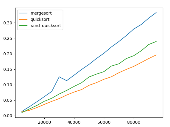
We see that randomization has some cost, but both versions of quicksort are significantly faster than merge sort. As we noted above, a further advantage of quicksort is that it runs in place.