We will use lists as a fundamental building block in our Python implementations of various algorithms, so it's important for us to understand how long various list operations will take. Suppose that l is a list with N elements. Then
Reading or writing l[i] will take O(1), for any i.
'x in l' will take O(1) in the best case (if x is is found immediately), or O(N) in the worst case (if x is not present, in which case Python has to scan all the way to the end of the list).
l.append(x) will take O(1) in the best case and O(N) in the worst case. It will run in O(1) in the average case. Specifically, if we begin with an empty list and append a value to it N times, then the total running time will be O(N), so the average time per append will be O(N) / N = O(1).
Why does append() not always run in O(1)? The answer is that when we append a value, Python must occasionally copy the entire list to a new memory area where there will be room for more values to be inserted. A Python list is essentially a dynamic array, which is an array that automatically grows when necessary. We will study this data structure and its performance later in this course.
'del l[0]', which deletes the first element of the list, will run in O(N), since all list elements must shift leftward. 'del l[-1]', which deletes the last list element, wlil run in O(1).
l.insert(0, x) will run in O(N), since all list elements must shift forward to make room for the new element.
Suppose that we begin with an empty list, and prepend a value to it N times by calling l.insert(0, x) in a loop. The total running time will be O(1 + 2 + … + N) = O(N2).
Notice that we can add and remove elements at the end of a list cheaply, but inserting and deleting at the beginning is relatively expensive.
Sorting is a fundamental task in computer science. Sorting an array means rearranging its elements so that they are in order from left to right.
We will study a variety of sorting algorithms in this class. Most of these algorithms will be comparison-based, meaning that they will work by comparing elements of the input array. And so they will work on sequences of any ordered data type: integer, real, string and so on. We will generally assume that any two elements can be compared in O(1).
Our first sorting algorithm is bubble sort. Bubble sort is not terribly efficient, but it is easy to write.
Bubble sort works by making a number of passes over the input array a. On each pass, it compares pairs of elements: first elements a[0] and a[1], then elements a[1] and a[2], and so on. After each comparison, it swaps the elements if they are out of order. Here is an animation of bubble sort in action.
Suppose that an array has N elements. Then the first pass of a bubble sort makes N – 1 comparisons, and always brings the largest element into the last position. So the second pass does not need to go as far: it makes only N – 2 comparisons, and brings the second-largest element into the second-to-last position. And so on. After N – 1 passes, the sort is complete and the array is in order.
Here's an implementation of bubble sort in Python:
def bubble_sort(a):
    n = len(a)
    for i in range(n - 1, 0, -1):   # n - 1 .. 1
        for j in range(i):
            if a[j] > a[j + 1]:
                a[j], a[j + 1] = a[j + 1], a[j]
What's the running time of bubble sort? Suppose that the input array has N elements. As mentioned above, on the first pass we make (N – 1) comparisons; on the second pass we make (N – 2) comparisons, and so on. The total number of comparisons is
(N – 1) + (N – 2) + … + 2 + 1 = N(N – 1) / 2 = O(N2)
The number of element swaps may also be O(N2), though it will be as low as 0 if the array is already sorted. In any case, the total running time is O(N2) in the best and worst case due to the cost of the comparisons.
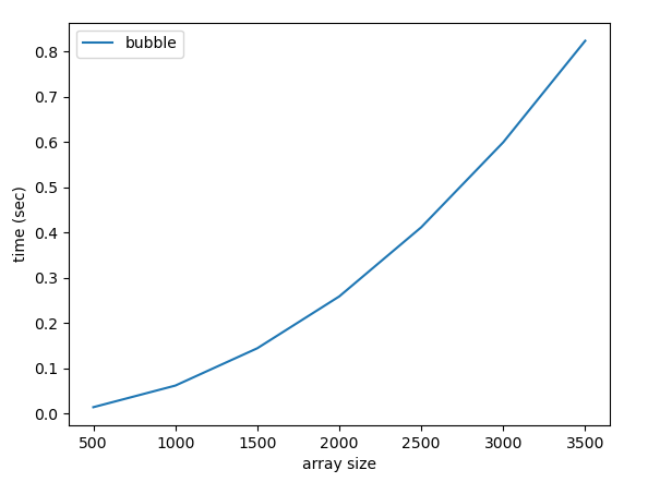
Let's generate a plot showing how bubble sort performs for various input sizes. The Python function time.time() returns a float representing the number of seconds that have elapsed since January 1, 1970. If we call this function both before and after sorting, then the difference in the returned times will indicate how long the sort took to run. Here is code to generate the plot:
import matplotlib.pyplot as plt
from random import randrange
import time
…
def test(n):
    a = []
    for i in range(n):
        a.append(randrange(1000))

    start = time.time()
    bubble(a)
    return time.time() - start

def plot():
    xs = range(500, 4000, 500)
    bub = []
    for n in xs:
        print(f'n = {n}')
        bub.append(test(n))

    plt.plot(xs, bub, label = 'bubble')
    plt.legend()
    plt.xlabel('array size')
    plt.ylabel('time (sec)')
    plt.show()
The plot looks like this:
The quadratic shape is evident.
Our next sorting algorithm is selection sort. In a selection sort, we start by finding the smallest value in the array and exchanging it with the first element. We then find the second smallest value and exchange it with the second element, and so on. Here is an animation of selection sort in action.
Here's an implementation in Python:
def selection_sort(a):
    n = len(a)
    for i in range(n - 1):
        min_index = i
        min_val = a[i]
        for j in range(i + 1, n):
            if a[j] < min_val:
                min_val = a[j]
                min_index = j
        a[i], a[min_index] = a[min_index], a[i]
We can analyze selection sort's running time similarly to bubble sort. Just as in bubble sort, the total number of comparisons is
(N – 1) + (N – 2) + … + 2 + 1 = N(N – 1) / 2 = O(N2)
and the running time is O(N2) in the best and worst case. However, selection sort will usually outperform bubble sort by as much as a factor of 3. That's because it performs many fewer swaps as it rearranges the data.
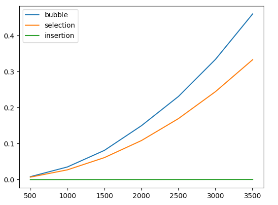
Let's extend the plot above to include a selection sort. To do that, we'll modify our test() function so that it takes an extra argument f indicating a sorting function to run. This is a feature of Python that we haven't seen yet: a variable or parameter can actually hold a function. (We will explore this concept more in a future lecture.)
# f is a sorting function
def test(n, f):
    a = []
    for i in range(n):
        a.append(randrange(1000))

    start = time.time()
    f(a)
    return time.time() - start

def plot():
    xs = range(500, 4000, 500)
    bub = []  # bubble
    sel = []  # selection
    for n in xs:
        print(f'n = {n}')
        bub.append(test(n, bubble))
        sel.append(test(n, selection))

    plt.plot(xs, bub, label = 'bubble')
    plt.plot(xs, sel, label = 'selection')
    plt.legend()
    plt.show()
Here is the result:

We can see that selection sort is significantly faster than bubble sort, perhaps by a factor of 2-3 in this Python implementation. However, selection sort is still evidently quadratic.
Insertion sort is another fundamental sorting algorithm. Insertion sort loops through array elements from left to right. For each element a[i], we first "lift" the element out of the array by saving it in a temporary variable t. We then walk leftward from i; as we go, we find all elements to the left of a[i] that are greater than a[i] and shift them rightward one position. This makes room so that we can insert a[i] to the left of those elements. And now the subarray a[0..i] is in sorted order. After we repeat this for all elements in turn, the entire array is sorted.
Here is an animation of insertion sort in action.
Here is a Python implementation of insertion sort:
def insertion_sort(a):
    n = len(a)
    for i in range(n):
        t = a[i]
        j = i - 1
        while j >= 0 and a[j] > t:
            a[j + 1] = a[j]
            j -= 1
        a[j + 1] = t
What is the running time of insertion sort? The worst case is when the input array is in reverse order. Then to insert each value we must shift elements to its left, so the total number of shifts is 1 + 2 + … + (n – 1) = O(n2). If the input array is ordered randomly, then on average we will shift half of the subarray elements on each iteration. Then the time is still O(n2).
In the best case, the input array is already sorted. Then no elements are shifted or modified at all and the algorithm runs in time O(n).
In summary, insertion sort has the same worst-case asymptotic running time as bubble sort and selection sort, i.e. O(n2). However, insertion sort has a major advantage over bubble sort and selection sort in that it is adaptive: when the input array is already sorted or nearly sorted, it runs especially quickly.
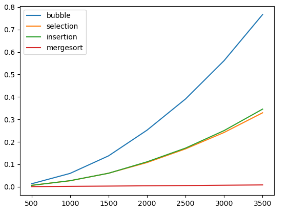
Let's extend our previous plot by adding insertion sort:

We see that on random data, selection sort and insertion sort behave quite similarly.
Now let's compare the running times of these algorithms on data that is already sorted:
As we can see, in this situation insertion sort is enormously faster. As we discussed above, with sorted input it runs in O(N) since no elements need to shift.
Suppose that we have two arrays, each of which contains a sorted sequence of integers. For example:
a = [3, 5, 8, 10, 12]
b = [6, 7, 11, 15, 18]
And suppose that we'd like to merge the numbers
in these arrays into a single array c
containing all of the numbers in sorted order.
A simple algorithm will
suffice. We can use integer variables i and j to point to members of
a and b, respectively. Initially i = j = 0. At each step of the
merge, we compare a[i]
and b[j].
If a[i] < b[j],
we copy a[i]
into the destination array, and increment i. Otherwise we copy b[j]
and increment j. The entire process will run in linear time, i.e. in
O(N) where N = len(a) + len(b).
Let's write a function to accomplish this task:
# Merge sorted arrays a and b into c, given that
# len(a) + len(b) = len(c).
def merge(a, b, c):
    i = j = 0     # index into a, b

    for k in range(len(c)):
        if j == len(b):      # no more elements available from b
            c[k] = a[i]      # so we take a[i]
            i += 1
        elif i == len(a):    # no more elements available from a
            c[k] = b[j]      # so we take b[j]
            j += 1
        elif a[i] < b[j]:
            c[k] = a[i]      # take a[i]
            i += 1
        else:
            c[k] = b[j]      # take b[j]
j += 1We can use this function to merge the arrays a and b mentioned above:
a = [3, 5, 8, 10, 12]
b = [6, 7, 11, 15, 18]
c = (len(a) + len(b)) * [0]

merge(a, b, c)
We now have a function that merges two sorted arrays. We can use this as the basis for implementing a sorting algorithm called merge sort.
Merge sort has a simple recursive structure. To sort an array of n elements, it divides the array in two and recursively merge sorts each half. It then merges the two sorted subarrays into a single sorted array.
For example, consider merge sort’s operation on this array:

Merge sort splits the array into two halves:

It then sorts each half, recursively.

Finally, it merges these two sorted arrays back into a single sorted array:

Here's an implemention of merge sort, using our merge() function from the previous section:
def merge_sort(a):
    if len(a) < 2:
        return

    mid = len(a) // 2

    left = a[:mid]      # copy of left half of array
    right = a[mid:]     # copy of right half

    merge_sort(left)
    merge_sort(right)

    merge(left, right, a)
Let's add merge sort to our performance graph, showing the time to sort random input data:
As we can see, merge sort is enormously faster than any of the other sorting methods that we have seen. Let's draw a plot showing the performance of only merge sort, with larger input sizes:
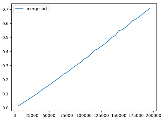
The performance looks nearly linear. In fact merge sort runs in O(N log N) in both the best and worst case. In the next lecture, we will see why this is the case.