You should all have seen the concept of limits in your high school mathematics courses. In computer science we are often concerned with limits as a variable goes to infinity. For example:
limx => ∞ (1 / x) = 0
limx => ∞ 3x / (x + 1) = 3
limx => ∞ (x + 2) / (sqrt(x) + 3) = ∞
We will say that a function f(n) grows faster than a function g(n) if the limit of f(n) / g(n) as n approaches ∞ is ∞. In other words, the ratio f(n) / g(n) becomes arbitrarily large as n increases. For example, n2 grows faster than 10n, since
limn => ∞ (n2 / 10n) = limn => ∞ (n / 10) = ∞
Here is a list of some common functions of n in increasing order. Each function in the list grows faster than all of its predecessors:
1
log (log n)
log n
sqrt(n)
n
n log n
n sqrt(n)
n2
n3
n4
2n
3n
n!
nn
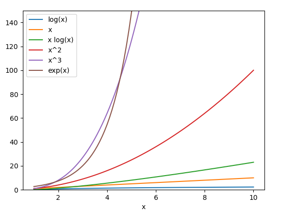
It would be nice to plot the functions listed above so that we can see how quickly they increase.
In this course and in Programming 1 we'll use the Matplotlib library for plotting. To install it on your machine, run the command
$ pip3 install matplotlib
To use Matplotlib in a Python program, import the matplotlib.pyplot package at the top of your source file. I recommend importing it using the convenient name 'plt':
import matplotlib.pyplot as plt
Our Python quick reference lists various useful Matplotlib methods.
Here's a Python program that will plot some of the functions above:
from math import exp, log
import matplotlib.pyplot as plt

XLIM = 10
YLIM = 150

xs = []
log_x = []
x_log_x = []
x_2 = []
x_3 = []
exp_x = []

x = 1
while x < XLIM:
    xs.append(x)
    log_x.append(log(x))
    x_log_x.append(x * log(x))
    x_2.append(x ** 2)
    x_3.append(x ** 3)
    exp_x.append(exp(x))
    x += 0.1

plt.figure(figsize = (8, 8))
plt.ylim(0, YLIM)

plt.xlabel('x')
plt.plot(xs, log_x, label = 'log(x)')
plt.plot(xs, xs, label = 'x')
plt.plot(xs, x_log_x, label = 'x log(x)')
plt.plot(xs, x_2, label = 'x^2')
plt.plot(xs, x_3, label = 'x^3')
plt.plot(xs, exp_x, label = 'exp(x)')

plt.legend()
plt.show()
It displays this graph:
The function exp(x) = ex will grow much faster than any polynomial function, though that's not obvious on this graph because it extends only to y = 150. Let's change YLIM to 10_000, then replot:
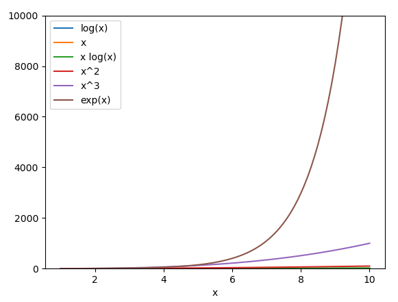
Now we can easily see that exp(x) will dominate all the other functions as x increases, though now the differences between some functions are hard to see because the vertical scale is so exaggerated.
We will define big-O notation as follows:
f(n) = O(g(n)) if limn => ∞ f(n) / g(n) = C for some 0 < C < ∞
This definition is actually a bit of a simplification since it does not cover cases in which the limit does not exist. However, it is adequate for our purposes for the moment. You may see a more general definition in ADS 1 next semester.
For example:
3 n2 + 7 n + 16 = O(n2) because limn => ∞ (3n2 + 7n + 16) / n2 = 3
5 n3 log n + n log n + 10 = O(n3 log n)
nn + n! + 2n = O(nn)
100 = O(1)
We see that we can write a function in big-O notation by discarding all lower-order terms, plus any constant factor.
We would like to consider how long our programs take to run as a function of their input size.
In general in this course we will assume that integer operations such as +, -, * and // run in constant time. (Strictly speaking, that is not true since integers in Python can be arbitrarily large. However, this is a common assumption that will make our analysis much easier.)
As a first example, consider this code, which computes a certain function of an input number n:
n = int(input('Enter n: '))
s = 0

for i in range(n):
  s += i

  for j in range(n):
    s += i * j

print('The answer is', s)
Here the input size is n. This code will run quickly when n is small, but as n increases the running time will certainly increase. How can we quantify this?
Here is the same code again, with comments indicating how many times each line will run:
n = int(input('Enter n: '))

s = 0                 # 1 time

for i in range(n):    # n times
  s += i              # n times

  for j in range(n):  # n * n times
    s += i * j        # n * n times

print('The answer is', s)
Suppose that the 5 commented statements above will run in times A, B, C, D, and E, where these letters are constants representing numbers of nanoseconds. Then the total running time is A + (B + C) n + (D + E) n2.
In theoretical computer science we don't care at all about the constant factors in an expression such as this. They are dependent on the particular machine on which a program runs, and may not even be so easy to determine. So we write:
running time = A + (B + C) n + (D + E) n2 = O(n2)
Coming back to our previous example, let's make a slight change to the code:
n = int(input('Enter n: '))

s = 0

for i in range(n):
  s += i

  for j in range(i):  # previously this was range(n)
    s += i * j

print('The answer is', s)
What is its running time now?
Once again the statement "s = 0" will execute once, and the statements "for i" and "s += i" will execute n times. The statements "for j" and "s += i * j" will execute 0 times on the first iteration of the outer loop (when i = 0), 1 time on the next iteration (when i = 1) and so on. The total number of times they will execute is
0 + 1 + 2 + … + (n – 1) = n (n – 1) / 2 = n2 / 2 – n / 2 = O(n2)
Thus, the code's asymptotic running time is still O(n2).
This example illustrates an important principle that we will see many times in the course, namely that
1 + 2 + 3 + … + N = O(N2)
Let's consider the running time of the algorithms on integers that we have already studied in this course.
First let's look at primality testing using trial division, which we saw in the last lecture:
from math import sqrt

n = int(input('Enter n: '))

prime = True
for i in range(2, int(sqrt(n)) + 1):
    if n % i == 0:
        prime = False
        break

if prime:
    print('n is prime')
else:
    print('not prime')
Notice that for this algorithm some values of n are harder than others. For example, if n is even then the function will exit immediately, even if n is very large. On the other hand, if n is prime then the function will need to iterate all the way up to sqrt(n) in order to determine its primality.
In general we are interested in determining an algorithm's best-case and worst-case running times as the input size n increases. For some algorithms these will be the same, and for others they will be different. The best-case running time is a lower bound on how long it might take the algorithm to run when n is large, and the worst-case running time is an upper bound.
Let's annotate the code above with the number of times each statement might run:
from math import sqrt

n = int(input('Enter n: '))

prime = True
for i in range(2, int(sqrt(n)) + 1):
    if n % i == 0:  # min = 1, max = sqrt(n) - 1
        prime = False
        break

if prime:
    print('n is prime')
else:
    print('not prime')
The statement "if
n % i == 0"
might run only once, or as many as sqrt(n) – 1 times.
This function runs in O(1) in the best case. That's because even when n is extremely large, the 'for' loop might exit immediately (e.g. if n is divisible by 2). The function runs in O(sqrt(n)) in the worst case.
Next, let's revisit our integer factorization algorithm:
from math import sqrt

n = int(input('Enter n: '))

f = 2
s = ''
while f <= int(sqrt(n)):
    if n % f == 0:  # n is divisible by f
        s += f'{f} * '
        n = n // f
    else:
        f += 1

s += str(n)     # append the last factor
print(s)
This is a bit trickier to analyze. In the worst case, n is prime, and the test 'if n % f == 0' will execute sqrt(n) – 1 times. Thus the worst-case running time is O(sqrt(n)).
Now suppose that n is a power of 2. Then the test 'if n % i == 0' will run log2 n – 1 times, and the program will run in O(log2 n) = O(log n). So the best-case running time is at most O(log n) (and might even be a bit less that that, though a precise analysis is beyond our discussion today).
For integers a and b, the greatest common divisor of a and b, also written as gcd(a, b), is the largest integer that evenly divides both a and b. For example:
gcd(20, 6) = 2
gcd(12, 18) = 6
gcd(35, 15) = 5
The greatest common divisor is useful in various situations, such as simplifying fractions. For example, suppose that we want to simplify 35/15. gcd(35, 15) = 5, so we can divide both the numerator and denominator by 5, yielding 7/3.
Naively, we can find the gcd of two values by trial division:
a = int(input('Enter a: '))
b = int(input('Enter b: '))

for i in range(min(a, b), 0, -1):
  if a % i == 0 and b % i == 0:
    break

print('The gcd is', i)
But this may take time O(N), where N = min(a, b). We'd like to be more efficient, especially since in some situations (e.g. cryptography) we may want to take the gcd of numbers that are very large.
Another way to find the greatest common divisor of two numbers is to factor the numbers into primes. For every prime p, if the prime factorization of a includes pi, and the prime factorization of b includes pj, then the prime factorization of gcd(a, b) will include pmin(i, j). (In other words, the prime factorization of gcd(a, b) is the intersection of the prime factorizations of a and b.)
For example consider finding gcd(252, 90). 252 = 9 * 28 = 22 * 32 * 71. And 90 = 9 * 10 = 21 * 32 * 51. So the common primes are 21 * 32 = 18, and we have gcd(252, 90) = 18.
Euclid’s algorithm is a much more efficient way to find the gcd of two numbers than prime factorization. It is based on the fact that for all positive integers a and b, gcd(a, b) = gcd(b, a mod b). (We will prove this below.) So, for example,
gcd(252, 90)
=
gcd(90, 72)
= gcd(72, 18)
= gcd(18, 0)
= 18
We can implement Euclid's algorithm in Python like this:
a = int(input('Enter a: '))
b = int(input('Enter b: '))

while b > 0:
  a, b = b, a % b

print('The gcd is', a)
Notice that the line "a, b = b, a % b" is a simultaneous assignment. You can read it like this: the new value of a is the previous value of b, and the new value of b is the previous value of (a % b).
In all the examples of gcd(a, b) above we had a > b. But note that this function works even when a < b ! For example, if we call gcd(5, 15), then on the first iteration of the while loop we have a % b = 5 mod 15 = 5. So then we assign a = 15 and b = 5, and further iterations continue as if we had called gcd(15, 5).
Above, we said that Euclid's algorithm works because of this mathematical fact: for all integers a and b,
gcd(a, b) = gcd(b, a mod b)
Let's now prove that. First, let's introduce the notion of a linear combination of two integers a and b, which is any integer of the form ia + jb for some integers i and j. For example, 26 is a linear combination of 3 and 5, because 2 · 3 + 4 · 5 = 26. To put it differently, a linear combination of a and b is any number that we can form by adding up some number of a's plus some number of b's.
The notation d | n means that d divides n, i.e. n is a multiple of d. Notice that if d | a and d | b, then d also divides any linear combination of a and b. For example, any linear combination of 6 and 10 must be divisible by 2, because 2 | 6 and 2 | 10.
We'd like to show that the sets {a, b} and {b, a mod b} have the same common divisors. Suppose that d | b and d | a mod b. We have already seen this equation that relates a, b, a div b and a mod b:
a = b · (a div b) + (a mod b)
We see that a is a linear combination of b and (a mod b). So we know that d | a. And so if d is a divisor of both b and (a mod b), then it's a divisor of both a and b.
Now suppose that d | a and d | b. We can rearrange the equation above to to
a mod b = a – b · (a div b)
We see that (a mod b) is a linear combination of a and b. So we know that d | (a mod b). And so if d is a divisor of both a and b, then it's a divisor of both b and (a mod b).
So the sets {a, b} and {b, a mod b} have the same common divisors. Therefore the sets have the same greatest common divisors, and so gcd(a, b) = gcd(b, a mod b).
We'd now like to consider the running time of Euclid's algorithm. Frst note that for any integers a, b with a > b, we have
(a mod b) < a / 2
For if 0 < b ≤ a / 2, then (a mod b) ≤ b – 1 < a / 2. Or if a / 2 < b < a, then a div b = 1, so (a mod b) = a – b < a – a / 2 = a / 2.
Now suppose that we call gcd(x, y) and the function runs for at least a few iterations. Then
iteration 1: a = x, b = y
iteration 2: a = y, b = (x mod y)
iteration 3: a = (x mod y), b = …
In two iterations the first argument has dropped from x to (x mod y), which is less than x / 2. So after every two iterations of the algorithm, the first argument will be reduced by at least a factor of 2. This shows that the algorithm cannot iterate more than 2 log2(x) times. In other words, it runs in time O(log N) in the worst case, since N = x.
We have seen how to compute the greatest common divisor of two integers A related concept is the least common multiple of two integers p and q, which is the smallest integer that is divisible by both p and q. For example,
lcm(60, 90) = 180
As with the gcd, we can find the least common multiple of two numbers by computing their prime factorizations. For every prime p, if the prime factorization of a includes pi, and the prime factorization of b includes pj, then the prime factorization of gcd(a, b) will include pmax(i, j). (In other words, the prime factorization of gcd(a, b) is the union of the prime factorizations of a and b.)
How can we compute a least common multiple efficiently? Here is a useful fact: for all integers and b,
gcd(a, b) · lcm(a, b) = a · b
Why is this true? First observe that for any integers i and j, trivially
min(i, j) + max(i, j) = i + j
Now, given integers a and b, consider any prime p. Suppose that the prime factorization of a contains pi, and the prime factorization of b contains pj. Then we have already seen that the prime factorization of gcd(a, b) contains pmin(i, j), and the prime factorization of lcm(a, b) contains pmax(i, j). Therefore the prime factorization of the product gcd(a, b) · lcm(a, b) will contain pmin(i, j) + max(i, j) = pi + j, which is also present in the prime factorization of the product a · b. Since this is true for all primes in the factorizations, we have gcd(a, b) · lcm(a, b) = a · b.
Now we can rearrange the formula above to give us lcm(a, b):
lcm(a, b) = a · b / gcd(a, b)
We can compute the gcd efficiently using Euclid's algorithm, so this formula gives us an efficient way to compute the lcm.