
In recent lectures we learned about stacks and queues, which are abstract data types that we can implement in various ways, such as using an array or a linked list.
A priority queue is another abstract data type. At a minimum, a priority queue might provide the following methods:
A priority queue differs from a stack and an ordinary queue in the
order in which elements are removed. A stack is last in first out:
the pop function removes the element that was added most
recently. An ordinary queue is first in first out: the dequeue
function removes the element that was added least recently. In a
priority queue, the remove_smallest() method
removes the element with the smallest
value.
The interface above describes a min-queue, in which we can efficiently remove the smallest value. Alternatively we can build a max-queue, which has a remove_largest() method that removes the largest value; this is more convenient for some applications. There is no fundamental differerence between these: any data structure that implements a min-queue can be trivially modified to produce a max-queue, by changing the direction of element comparisons.
In theory we could implement a priority queue using a binary search tree. If we did so and the tree was balanced, then add() and remove_smallest() would run in time O(log N), where N is the number of elements in the queue. But there are more efficient data structures for implementing priority queues, such as binary heaps, which we will now discuss.
Every node is smaller than or equal to its children. To be more precise, if a node with value p has a child with value c, then p ≤ c. This is sometimes called the heap property.
All levels of the tree are complete except possibly the last level, which may be missing some nodes on the right side.
For example, here is a binary heap:
This heap looks like a complete binary tree with one node missing on the right in the last level.
The height of a binary heap with N nodes is ⌊log2(N)⌋ = O(log N). In other words, a binary heap is always balanced.
We don’t store a binary heap using dynamically
allocated nodes and pointers. Instead, we use an array, which
is more compact, and is possible because of the shape of the binary
heap tree structure. The binary heap above can be stored in an array
like this:
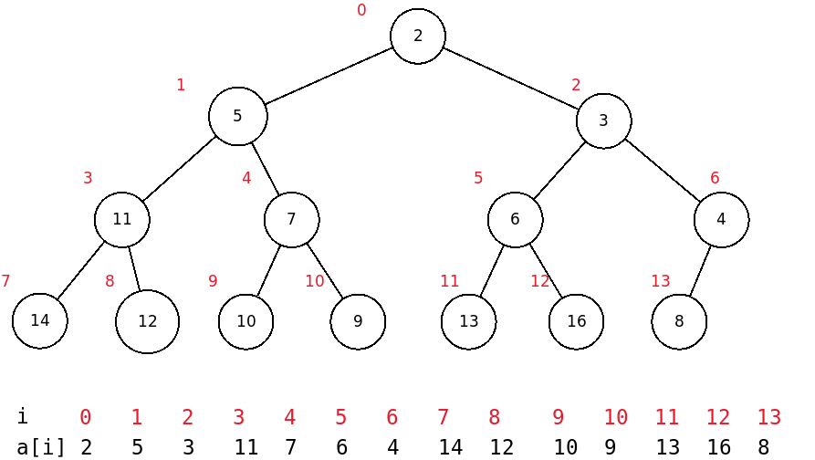
Notice that the array values are in the same order in which they appear in the tree, reading across tree levels from top to bottom and left to right.
From the tree above we can see the following patterns. If a heap node N has index i, then
N’s left child (if any) has index 2i + 1
N’s right child (if any) has index 2i + 2
N’s parent (if any) has index (i - 1) div 2
In Python, we can store heap elements in an ordinary Python list (which, as we know, is actually a dynamically sizeable array):
class BinaryHeap:
    def __init__(self):
        self.a = []    # list will hold heap elements
Let's write helper functions that move between related tree nodes, using the formulas we saw above:
def left(i):
    return 2 * i + 1

def right(i):
    return 2 * i + 2

def parent(i):
    return (i - 1) // 2
The heap depicted above is a min-heap, which supports a remove_smallest() operation. If we like, we may trivially modify it to be a max-heap, which instead supports a remove_largest() operation. In a max-heap, every node has a value that is larger than its children, and the largest value is at the top.
We will now describe operations that will let us use a min-heap as a priority queue.
We first consider inserting a value v into a heap. To do this, we first add v to the end of the heap array, expanding the array size by 1. Now v is in a new leaf node at the end of the last heap level. The heap still has a valid shape, except that it may be invalid since one node (the node we just added) may have a value v that is smaller than its parent.
So we now perform an operation called up heap, which will move v upward if necessary to restore the heap properties. Suppose that v’s parent has value p, and p > v. That parent may have a second child with value w. We begin by swapping the values v and p. Now v’s children are p and w (if present). We know that v < p. If w is present then p < w, so v < w by transitivity. Thus the heap properties have been restored for the node that now contains v. And now we continue this process, swapping v upward in the heap until it reaches a position where it is not larger than its parent, or until it reaches the root of the tree.
In Python, the insert operation will look like this:
    # in class BinaryHeap

    def up_heap(self, i):
        while i > 0:
            p = parent(i)
            if self.a[p] <= self.a[i]:
                break
            self.a[i], self.a[p] = self.a[p], self.a[i]
            i = p

    def insert(self, x):
        self.a.append(x)
        self.up_heap(len(self.a) – 1)
The worst-case running time of an up heap operation is O(log N), since it will travel through O(log N) nodes at most (i.e. up to the top of the tree), and performs O(1) work at each step. And so insert() also runs in O(log N) in the worst case.
Now we consider removing the smallest value from a min-heap. Since the smallest value in such a heap is always in the root node, we must place some other value there. So we take the value at the end of the heap array and place it in the root, decreasing the array size by 1 as we do so. Now the heap still has a valid shape, however it may be invalid since its value at the root may be larger than one or both of its children.
So we now perform an operation called down heap on this value v, which will lower it to a valid position in the tree. If v is larger than one or both of its children, then let w be the value of the smallest of v's children. Then we know that v > w. We swap v with w. Now w's children are v and possibly some other value x. We know that w < v, and if there is another child x then w < x, since w was the smallest child. So the heap property has been restored for the node that now contains w. We then continue this process, swapping v downward as many times as necessary until v reaches a point where it has no larger children. The process is guaranteed to terminate successfully, since if v eventually descends to a leaf node there will be no children and the condition will be satisfied.
In Python, remove_smallest() will look like this:
 def down_heap(self, i):
        while True:
            l, r = left(i), right(i)

            # Find the index (i, l, or r) with the smallest value.
            j = i
            if l < len(self.a) and self.a[l] < self.a[j]:   # left child exists and is smaller
                j = l
            if r < len(self.a) and self.a[r] < self.a[j]:   # right child exists and is smaller
                j = r

            if j == i:  # i is smaller than any of its children
                break
            self.a[i], self.a[j] = self.a[j], self.a[i]
            i = j

def remove_smallest(self):
        x = self.a[0]
        self.a[0] = self.a.pop()
        self.down_heap(0)
        return x
Similarly to an up heap operation, the running time of a down heap operation is O(log N) in the worst case, since it will travel through O(log N) nodes at most (i.e. up to the top of the tree), and performs O(1) work at each step. And so remove_smallest() also runs in O(log N) in the worst case.
Suppose that we have an array a of numbers in any order, and we'd like to heapify the array, i.e. rearrange its elements so that they form a valid binary heap. How can we do this?
One possible approach would to iterate over the array elements from left to right, performing an up heap operation on each one. After each such operation, the array elements visited so far will be a valid binary heap, so when we are done we will have a valid heap containing all array elements. If there are N elements in the array, then there may be as many as N / 2 leaf nodes. The up heap operation on each leaf may take O(log N) time, since it may travel all the way up the tree. Thus, in the worst case the heapification may take N / 2 · O(log N) = O(N log N).
However, there is a better way. We can instead iterate over the array elements from right to left, performing a down heap operation on each one. At each step, the heap property will be valid for all nodes that we've already visited, so when we're done will have a complete valid binary heap.
How long will this take? Suppose that there are N elements in the array. For simplicity, let's assume that N = 2k – 1 for some k, so that the heap has the form of a complete binary tree with height (k - 1). Then there are 2k – 1 leaves, which is approximately N / 2. We don't even need to perform a down heap operation on these, since there is nothing below them. There are 2k – 2 parents of leaves, which is approximately (N / 4). The down heap operation on each of these will take only one step, since each such node will fall at one most position. So the total running time will be proportional to
0 · (N / 2) + 1 · (N / 4) + 2 · (N / 8) + 3 · (N / 16) + …
Let's rewrite the expression above in a two-dimensional form:
N / 4 + N / 8 + N / 16 + N / 32 + N / 64 + …
      + N / 8 + N / 16 + N / 32 + N / 64 + …
               + N / 16 + N / 32 + N / 64 + …
                       + N / 32 + N / 64 + …

                        + …
The sum of the first row above is N / 2. The sum of the second row is N / 4, and so on. The total of all rows is
N / 2 + N / 4 + N / 8 + … = N
Thus the total cost of this heapification process is O(N). It is remarkably efficient.
We’ve already seen several sorting algorithms in this course: bubble sort, selection sort, insertion sort, merge sort and quicksort. We can use a binary heap to implement yet another sorting algorithm: heapsort. The essence of heapsort is simple: given a array of numbers to sort, we put them into a heap, and then we pull out the numbers one by one in sorted order.
Let’s examine these steps in a more detail. For
heapsort, we want a max-heap, which lets us remove the largest
element by calling a method remove_largest.
Given an array of N values, we first heapify it as described
above. After that, sorting the array is easy: we repeatedly call
remove_largest
to remove the largest element, which we place at the end of the
array, to the left of any other elements that we have already
removed. When we are done, the array will be sorted. A Python
implementation will look like this:
class Heap:
    def __init__(self, a):
        self.a = a
        self.n = len(a)  # current heap size

        # Heapify the given array.
        for i in range(self.n - 1, -1, -1):
            self.down_heap(i)

    def down_heap(self, i):
        while True:
            l, r = left(i), right(i)
            j = i
            if l < self.n and self.a[l] > self.a[j]:
                j = l
            if r < self.n and self.a[r] > self.a[j]:
                j = r
            if j == i:
                break
            self.a[i], self.a[j] = self.a[j], self.a[i]
            i = j

    def remove_largest(self):
        x = self.a[0]
        self.a[0] = self.a[self.n - 1]
        self.n -= 1
        self.down_heap(0)
        return x

    def sort(self):
        while self.n > 0:
            x = self.remove_largest()
            self.a[self.n] = x

def heapsort(a):
    h = Heap(a)
    h.sort()
The total time for heapsort to sort N values is (a) the time to heapify the array plus (b) the time to remove each of the N values from the heap in turn. This is
O(N) + O(N log N) = O(N log N)
Thus heapsort has the same asymptotic running time as merge sort and quicksort. Some advantages of heapsort are that it runs on an array in place (unlike merge sort) and that it is guaranteed to run in time O(N log N) for any input (unlike quicksort).
Here is a graph showing the relative performance of our Python implementations of merge sort, quicksort, and heapsort on random arrays containing up to 100,000 elements. Both randomized and non-randomized versions of quicksort are shown:

We can see that heapsort is substantially slower than quicksort. Nevertheless, it is sometimes used in environments where memory is limited and quicksort's worst-case quadratic behavior would be unacceptable. For example, the Linux kernel uses heapsort internally. Another advantage of heapsort is that its implementation is non-recursive, so there is no danger of overflowing the call stack, as could happen in quicksort with a worst-case input.
We have studied 6 different sorting algorithms in this class! Three of them (bubble sort, selection sort, insertion sort) run in O(N2) time in the worst case, and three of them (merge sort, quick sort, bubble sort) typically run in O(N log N). All six of these algorithms are comparison-based, i.e. they work by making a series of comparisons between values in the input array.
We will now ask: is there any sorting algorithm that can sort N values in time better than O(N log N) in the worst case? We will show that for any comparison-based sorting algorithm, the answer is no: O(N log N) is the fastest time that is possible.
Any comparison-based sorting algorithm makes a series of comparisons, which we may represent in a decision tree. Once it is has performed enough comparisons, it knows how the input values are ordered.
For example, consider an input array with three elements a, b, and c. One possible comparison-based algorithm might compare the input elements following this decision tree:
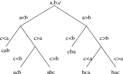
The algorithm first compares a and b. If a < b, it then compares a and c. If c < a, then the algorithm now knows a complete ordering of the input elements: it is c < a < b. And presumably as the algorithm runs it will rearrange the array elements into this order.
This algorithm will perform 2 comparisons in the best case. In the worst case, it will perform 3 comparisons, since the height of the tree above is 3.
Might it be possible to write a comparison-based algorithm that determines the ordering of 3 elements using only 2 comparisons in the worst case? The answer is no. With only 2 comparisons, the height of the decision tree will be 2, which means that it will have at most 22 = 4 leaves. However there are 3! = 6 possible permutations of 3 elements, so a decision tree with height 2 is not sufficient to distinguish them all.
More generally, suppose that we are sorting an array with N elements. There are N! possible orderings of these elements. If we want to distinguish all these orderings with k comparisons, then our decision tree will have at most 2k leaves, and so we must have
2k ≥ N!
or
k ≥ log2(N!)
We may approximate N! using Stirling's formula, which says that
N! ~ sqrt(2 π N) (N / e)N
And so we have
k >= log2(N!)
= log2(sqrt(2 π N) (N / e)N)
= log2(sqrt(2 π N)) + log2((N / e)N)
= 0.5 (log2(2) + log2(π) + log2(N)) + N (log2(N) – log2(e))
= O(N log N)
This shows that any comparison-based sorting algorithm will require O(N log N) comparisons in the worst case, and thus will run in time at least O(N log N).