Introduction to Algorithms, 2021-2
Week 14: Notes

Some of this week's topics are covered in Problem Solving with Algorithms:

• 4.9 Infix, Prefix and Postfix Expressions

And in Introduction to Algorithms:

• 8. Sorting in Linear Time

Here are some additional notes.

expression trees

In the last lecture, we discussed infix, prefix, and postfix forms of arithmetic expressions. We will now discuss how to store and work with arithmetic expressions in a program.

We may store expressions using an expression tree, which is a form of abstract syntax tree. An expression tree reflects an expression’s hierarchical structure. For example, here is an expression tree for the infix expression ((3 + 4) * (2 + 5)):

Note that this expression tree also corresponds to the prefix expression * + 3 4 + 2 5, or the postfix expression 3 4 + 2 5 + *. Equivalent expressions in infix, prefix or postfix form will always have the same tree! That’s because this tree reflects the abstract syntax of the expression, which is independent of concrete syntax which defines how expressions are written as strings of symbols.

We can easily store expression trees using objects in Python. Every interior node of the tree represents a binary operation, and every leaf is an integer. Here is a class for interior nodes:

class OpExpr:
    def __init__(self, op, left, right):
        self.op = op     # character, e.g. '+'
        self.left = left
        self.right = right

This may remind you of the class for binary search trees that we saw a few weeks ago. However, note some important differences. In our representation of binary search trees, we held values (typically numbers) in every node, and the left and right children of every left node were None. In these expression trees, the leaves are Python integers.

We can build the expression tree in the picture above as follows:

l = OpExpr('+', 3, 4)
r = OpExpr('+', 2, 5)
top = OpExpr('*', l, r)

grammar for arithmetic expressions

We will now formally define the syntax of arithmetic expressions, which will help us in the next section when we write a parser.

For simplicity, we will assume that

• all numbers consist of only a single digit

• the only operators are +, -, *, / meaning integer addition, subtraction, multiplication and division

• expressions have no embedded spaces

For now, we will consider arithmetic expressions in prefix form. We can define the syntax of prefix arithmetic expressions using the following context-free grammar:

digit → '0' | '1' | '2' | '3' | '4' | '5' | '6' | '7' | '8' | '9'
op → '+' | '-' | '*' | '/'
expr → digit | op expr expr

Context-free grammars are commonly used to define programming languages. A grammar contains non-terminal symbols (such as digit, op, expr) and terminal symbols (such as '0', '1', '2', …, '+', '-', '*', '/'), which are characters. A grammar consists of a set of production rules that define how each non-terminal symbol can be constructed from other symbols. These rules collectively define which strings of terminal symbols are syntactically valid.

For example, * + 4 5 9 is a valid prefix expression in the syntax defined by this grammar, because it can be constructed from the top-level non-terminal expr by successively replacing symbols using the production rules:

expr
→ op expr expr
→ op op expr expr expr
→ * + digit digit digit
→ * + 4 5 9

You will learn more about context-free grammars in more advanced courses.

parsing prefix expressions

We would now like to parse prefix arithmetic expressions defined by the grammar above. Specifically, given a string containing a prefix expression, we'd like to be able to convert it into an abstract syntax tree in memory.

We will need to read characters one at a time from a string. So let's first write a class Reader that lets us do that:

class Reader:
    def __init__(self, s):
        self.s = s.replace(' ', '')     # ignore spaces
        self.pos = 0
    
    def read(self):
        assert self.pos < len(self.s)
        c = self.s[self.pos]
        self.pos += 1
        return c

It works:

>>> r = Reader('+ 2 3')
>>> r.read()
'+'
>>> r.read()
'2'
>>> r.read()
'3'

>>>

Let's write a function that can parse an arithmetic expression in prefix notation and generate an expression tree.

def parse_prefix(s):
    r = Reader(s)

    def parse():
        c = r.read()
        if '0' <= c <= '9':
            return int(c)
        
        if c in '+-*/':
            left = parse()
            right = parse()
            return OpExpr(c, left, right)

        assert False, 'syntax error'

    return parse()

Notice that the structure of the recursive helper function parse() follows the grammar rule for prefix expressions:

expr → digit | op expr expr

Let's try the parser:

>>> e = parse_prefix('+ * 2 3 4')
>>> e.op
'+'
>>> e.left.op
'*'
>>> e.left.left
2
>>> e.left.right
3
>>>

We have written a recursive-descent parser for an extremely simple language, i.e. the language of arithmetic expressions with operators +, -, *, / in prefix notation. Many interpreters and compilers for real programming languages such as Python also parse code using recursive-descent parsers, though of course those languages are far more complex.

evaluating an expression

If we have an expression tree in memory, we may wish to evaluate it, which means to determine its value. For example, when we evaluate the prefix expression + 2 * 3 4 , we get the value 14.

We will first write a function that can apply an operator to two numbers:

def eval_op(x, op, y):
    if op == '+': return x + y
    if op == '-': return x - y
    if op == '*': return x * y
    if op == '/': return x // y
    assert False, 'unknown operator: ' + op

Now we can evaluate an expression tree with a straightforward recursive function:

def eval(e):
    if isinstance(e, int):
        return e
    
    if isinstance(e, OpExpr):
        l = eval(e.left)
        r = eval(e.right)
        return eval_op(l, e.op, r)

    assert False, 'error'

Let's try it out:

>>> e = parse_prefix('+ 2 * 3 4')
>>> eval(e)
14
>>>

converting back to prefix form

Given an expression tree, it’s not hard to convert it to a string representation. For example, we can generate a prefix expression as follows:

def to_prefix(e):
    if isinstance(e, int):
        return str(e)
    
    if isinstance(e, OpExpr):
        left = to_prefix(e.left)
        right = to_prefix(e.right)
        return f'{e.op} {left} {right}'

    assert false, 'error'

Let's try it:

>>> e = parse_prefix('+ 2 * 3 4')
>>> to_prefix(e)
'+ 2 * 3 4'
>>>

If we like, we may easily modify this function to generate an expression in infix or postfix form instead.

parsing an infix expression

Above, we saw how to parse expressions in prefix form. Parsing an infix expression is not much more difficult. Let's first write a context-free grammar for the infix expressions that we wish to parse:

digit → '0' | '1' | '2' | '3' | '4' | '5' | '6' | '7' | '8' | '9'
op → '+' | '-' | '*' | '/'
expr → digit | '(' expr op expr ')'

Notice that in this grammar, all expressions must be fully parenthesized. That is to say, whenever we apply an operator to two operands, we must place parentheses around the result. This ensures that our grammar is unambiguous.

We now write a recursive function that mirrors this rule:

def parse_infix(s):
    r = Reader(s)

    def parse():
        c = r.read()
        if '0' <= c <= '9':
            return int(c)
        
        if c == '(':
            left = parse()
            op = r.read()
            right = parse()
            assert r.read() == ')', 'syntax error'
            return OpExpr(op, left, right)

        assert False, 'syntax error'

    return parse()

Just as when we wrote a prefix parser above, the structure of the parse() function closely follows the associated grammar rule.

Once we have parsed an infix expression, we can easily evaluate it, or convert to a prefix representation:

>>> e = parse_infix('((2 + 3) * (4 + 5))')
>>> eval(e)
45
>>> to_prefix(e)
'* + 2 3 + 4 5'

parsing a postfix expression

In this lecture we did not had time to discuss how to parse an expression in postfix form. Briefly, a recursive descent parser will not work for this sort of expression; instead, we need to use a stack. Each time the parser sees an integer constant, it will push it to the stack. When it sees an operator character, it will pop two expressions from the stack and push an OpExpr that combines them. When it has read the entire input string, the stack will contain a single value, namely an expression tree for the entire input expression. You may wish to think about this more and attempt to implement a postfix expression parser as an exercise.

lower bounds for sorting

Let's return to the topic of sorting. We have studied 6 different sorting algorithms in this class! Three of them (bubble sort, selection sort, insertion sort) run in O(N²) time in the worst case, and three of them (merge sort, quick sort, bubble sort) typically run in O(N log N).

This leads to the following question: is there any sorting algorithm that can sort N values in time better than O(N log N) in the worst case?

We will demonstrate that for any comparison-based sorting algorithm, the answer is no: O(N log N) is the fastest time that is possible. A comparison-based sorting algorithm is one that works by making a series of comparisons between values in the input array. All six of the sorting algorithms above are comparison-based.

We can imagine that any comparison-based sorting algorithm makes a series of comparisons, which we may represent in a decision tree. Once it is has performed enough comparisons, it knows how the input values are ordered.

For example, consider an input array with three elements a, b, and c. One possible comparison-based algorithm might compare the input elements following this decision tree:

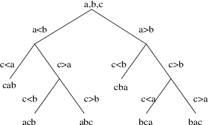
The algorithm first compares a and b. If a < b, it then compares a and c. If c < a, then the algorithm now knows a complete ordering of the input elements: it is c < a < b. And presumably as the algorithm runs it will rearrange the array elements into this order.

This algorithm will perform 2 comparisons in the best case. In the worst case, it will perform 3 comparisons, since the height of the tree above is 3.

Might it be possible to write a comparison-based algorithm that determines the ordering of 3 elements using only 2 comparisons in the worst case? The answer is no. With only 2 comparisons, the height of the decision tree will be 2, which means that it will have at most 2² = 4 leaves. However there are 3! = 6 possible permutations of 3 elements, so a decision tree with height 2 is not sufficient to distinguish them all.

More generally, suppose that we are sorting an array with N elements. There are N! possible orderings of these elements. If we want to distinguish all these orderings with k comparisons, then our decision tree will have at most 2^k leaves, and so we have

2^k >= N!

or

k >= log₂(N!)

We may approximate N! using Stirling's formula, which says that

N! ~ sqrt(2 π N) (N / e)^N

And so we have

k >= log₂(N!)

= log₂(sqrt(2 π N) (N / e)^N)

= log₂(sqrt(2 π N)) + log₂((N / e)^N)

= 0.5 (log₂(2) + log₂(π) + log₂(N)) + N (log₂(N) – log₂(e))

= O(N log N)

This shows that any comparison-based sorting algorithm will require O(N log N) comparisons in the worst case, and thus will run in time at least O(N log N).

sorting in linear time

Despite the result of the previous section, there do exist some sorting algorithms that can run in linear time! These algorithms are not comparison-based, and so they are not as general as the other sorting algorithms we've studied in this course. In other words, they will work only on certain types of input data.

Let's study one linear-time sorting algorithm, namely counting sort. In its simplest form, counting sort works on an input array of integers in the range 0 .. (M – 1) for some fixed integer M. The algorithm traverses the input array and builds a table that maps each integer k (0 <= k < M) to a value count[k] indicating how many times it occurred in the input. After that, it makes a second pass over the input array, writing each integer k exactly count[k] times as it does so.

For example, suppose that M = 5 and the input array is

2 4 0 1 2 1 4 4 2 0

The table of counts will look like this:

• count[0] = 2

• count[1] = 2

• count[2] = 3

• count[3] = 0

• count[4] = 3

So during the second pass the algorithm will write two 0s, two 1s, three 2s and so on. The result will be

0 0 1 1 2 2 2 4 4 4

Here is an implementation:

# Sort the array a, which contains integers in the range 0 .. (m - 1).
def counting_sort(a, m):
    count = m * [0]

    for x in a:
        count[x] += 1

    pos = 0
    for k in range(m):
        for i in range(count[k]):
            a[pos] = k
            pos += 1
    

Let's consider the running time of this function. All values in the input are known to be less than M. Let N be the length of the input array a. Then it will take time O(M) to allocate the array 'count', as well as to examine each of its values in the second pass. It will take time O(N) to read each value from the input array and to write new values into the array on the second pass. The total running time will be O(M + N). If we consider M to be a constant, this is O(N).

Of course, if M is large (such as the typical values 2³² or 2⁶⁴) then the algorithm will be slow and use an enormous amount of memory. In later classes you may see more advanced linear-time sorting algorithms such as radix sort, which can efficiently sort even integers in a large range.