Some of today's topics are covered in these sections of Problem Solving with Algorithms:
Recursion
Searching and Sorting
Sorting
And in Introduction to Algorithms:
2. Getting Started
2.3 Designing algorithms (describes mergesort)
Here are some additional notes on all of these topics.
A recursive function calls itself. Recursion is a powerful technique that can help us solve many problems.
As a first example, consider the implementation of Euclid's algorithm that we saw in an earlier lecture:
# gcd, iteratively
def gcd(a, b):
  while b > 0:
    a, b = b, a % b
  return a
We can rewrite this function using recursion:
# gcd, recursively
def gcd1(a, b):
  if b == 0:
    return a

  return gcd(b, a % b)
Whenever we write a recursive function, there is a base case and a recursive case.
The base case is an instance that we can solve immediately. In the function above, the base case is when b == 0. A recursive function must always have a base case – otherwise it would loop forever since it would always call itself.
In the recursive case, a function calls itself recursively,
passing it a smaller instance of the given problem. Then it
uses the return value from the recursive call to construct a value
that it itself can return. In the recursive case in this example, we
call gcd(b, a % b)
and return the value that it returns.
We have seen that we can write Euclid's algorithm either iteratively (i.e. using loops) or recursively. In theory, any function can be written either iteratively or recursively. We will see that for some problems a recursive solution is easy and an iterative solution would be quite difficult. Conversely, some problems are easier to solve iteratively. Python lets us write functions either way. (By the way, in purely functional languages such as Haskell there are no loops or iteration, so you must always use recursion. But that is a topic for another course.)
Broadly speaking, we will see
that "easy" recursive functions such as gcd
call themselves only once, and it
would be straightforward to write them either iteratively or
recursively. Soon
we will see recursive
functions that call themselves two or more times. Those functions
will let us solve more difficult tasks that we could not easily solve
iteratively.
For now, here is another example, a recursive procedure:
def hi(x):
  if x == 0:
    print('hi')
    return

  print('start', x)
  hi(x - 1)
  print('done', x)
If we call hi(3), the output will be
start 3
start 2
start 1
hi
done 1
done 2
done 3
Be sure you understand why the lines beginning with 'done' are printed. hi(3) calls hi(2), which calls hi(1), which calls hi(0). At the moment that hi(0) runs, all of these function invocations are active and are present in memory on the call stack:
hi(3)
→ hi(2)
  → hi(1)
    → hi(0)
Each function invocation has its own value of the parameter x. (If this procedure had local variables, each invocation would have a separate set of variable values as well.)
When hi(0) returns, it does not exit from this entire set of calls. It returns to its caller, i.e. hi(1). hi(1) now resumes execution and writes 'done 1'. Then it returns to hi(2), which writes 'done 2', and so on.
Here is another recursive function:
def sum_n(n):
  if n == 0:
    return 0

  return n + sum_n(n - 1)
What does this function do? Suppose that we call sum(3). It will call sum(2), which calls sum(1), which calls sum(0). The call stack now looks like this:
sum(3)
→ sum(2)
  → sum(1)
    → sum(0)
Now
sum(0) returns 0 to its caller sum(1).
sum(1) takes this value 0, adds n = 1 to it and returns 1 to sum(2).
sum(2) takes this value 1, adds n = 2 to it and returns 3 to sum(3).
sum(3) takes this value 3, adds n = 3 to it and returns 6.
We see that given any n, the function returns the sum 1 + 2 + 3 + … + n.
We were given this function and had to figure out what it does. But more often we will go in the other direction: given some problem, we'd like to write a recursive function to solve it. How can we do that?
Here is some general advice. To write any recursive function, first look for base case(s) where the function can return immediately. (As we will soon see, a function may sometimes have more than one base case.) Now you need to write the recursive case, where the function calls itself. At this point you may wish to pretend that the function "already works". Write the recursive call and believe that it will return a correct solution to a subproblem, i.e. a smaller instance of the problem. Now you must somehow transform that subproblem solution into a solution to the entire problem, and return it. This is really the key step: understanding the recursive structure of the problem, i.e. how a solution can be derived from a subproblem solution.
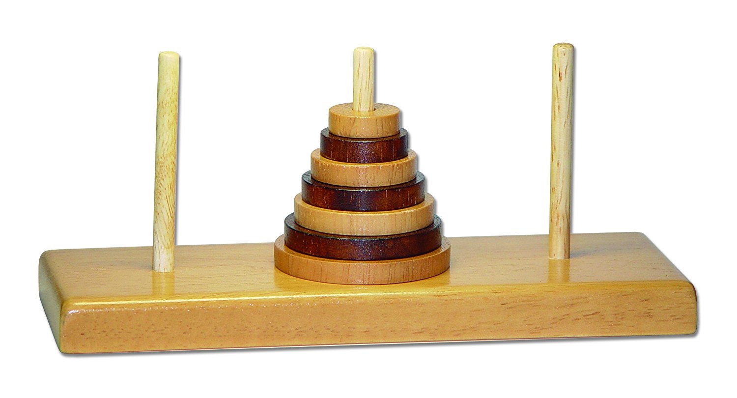
The Tower of Hanoi is a well-known puzzle that looks like this:
The puzzle has 3 pegs and a number of disks of various sizes. The player may move disks from peg to peg, but a larger disk may never rest atop a smaller one. Traditionally all disks begin on the leftmost peg, and the goal is to move them to the rightmost.
Supposedly in a temple in the city of Hanoi there is a real-life version of this puzzle with 3 rods and 64 golden disks. The monks there move one disk each second from one rod to another. When they finally succeed in moving all the disks to their destination, the world will end.
The world has not yet ended, so we can write a program that solves a version of this puzzle with a smaller number of disks. We want our program to print output like this:
move disk 1 from 1 to 2
move disk 2 from 1 to 3
move disk 1 from 2 to 3
move disk 3 from 1 to 2
…
To solve this puzzle, the key insight is that a simple recursive algorithm will do the trick. To move a tower of disks 1 through N from peg A to peg B, we can do the following:
Move the tower of disks 1 through N-1 from A to C.
Move disk N from A to B.
Move the tower of disks 1 through N-1 from C to B.
The program below implements this algorithm:
# move tower of n disks from fromPeg to toPeg
def hanoi(n, fromPeg = 1, toPeg = 3):
  if n == 0:
    return
  other = 6 - fromPeg - toPeg
  hanoi(n - 1, fromPeg, other)
  print(f'move disk {n} from {fromPeg} to {toPeg}')
  hanoi(n - 1, other, toPeg)
We can compute the exact number of moves required to solve the puzzle using the algorithm above. If M(n) is the number of moves to move a tower of height n, then we have the recurrence
M(n) = 2 ⋅ M(n–1) + 1
The solution to this recurrence is, exactly,
M(n) = 2n – 1
Similarly, the running time of our program above follows the recurrence
T(n) = 2 ⋅ T(n–1) + O(1)
And the program runs in time T(n) = O(2n).
It will take 264 - 1 seconds for the monks in Hanoi to move the golden disks to their destination tower. That is far more than the number of seconds that our universe has existed so far.
Suppose that we have two arrays, each of which contains a sorted sequence of integers. For example:
a = [3, 5, 8, 10, 12]
b = [6, 7, 11, 15, 18]
And suppose that we'd like to merge the numbers
in these arrays into a single array c
containing all of the numbers in sorted order.
Fortunately this is not difficult. We can
use integer variables i and j to point to members of a and b,
respectively. Initially i = j = 0. At each step of the merge, we
campare a[i]
and b[j].
If a[i] < b[j],
we copy a[i]
into the destination array, and increment i. Otherwise we copy b[j]
and increment j. The entire process will run in linear time, i.e. in
O(N) where N = len(a) + len(b).
Let's write a function to accomplish this task:
# Merge sorted arrays a and b onto c, given that
# len(a) + len(b) = len(c).
def merge(a, b, c):
  i = 0   # index into a
  j = 0   # index into b

  for k in range(len(c)):
    if j == len(b):    # j is out of bounds
      c[k] = a[i]      # so we take a[i]
      i += 1
    elif i == len(a):  # i is out of bounds
      c[k] = b[j]      # so we take b[j]
      j += 1
    elif a[i] < b[j]:  # both i and j are in bounds
      c[k] = a[i]
      i += 1
    else:
      c[k] = b[j]
      j += 1
Now we can use merge to merge the arrays a and b
mentioned above:
a = [3, 5, 8, 10, 12]
b = [6, 7, 11, 15, 18]
c = (len(a) + len(b)) * [0]

merge(a, b, c)
We now have a function that merges two sorted arrays. We can use this as the basis for implementing a general-purpose sorting algorithm called mergesort.
Mergesort has a simple recursive structure. To sort an array of n elements, it divides the array in two and recursively mergesorts each half. It then merged the two sorted subarrays into a single sorted array. This problem solving approach is called divide and conquer.
For example, consider mergesort’s operation on this array:

Merge sort splits the array into two halves:

It then sorts each half, recursively.

Finally, it merges these two sorted arrays back into a single sorted array:

Here's an animation of mergesort in action on the above array.
Here's
an implemention of mergesort, using our merge
procedure
from above:
def mergesort(a):
  if len(a) < 2:
    return

  mid = len(a) // 2

  left = a[:mid]
  mergesort(left)

  right = a[mid:]
  mergesort(right)

  merge(left, right, a)
What is the running time of mergesort? The helper
function merge runs in time O(N), where N is the length
of the array c. The array slice operations a[:mid] and a[mid:] also
take O(N). So the running time of mergesort follows the
recurrence
T(N) = 2 ⋅ T(N / 2) + O(N)
We have not seen this recurrence before. In this class we will not formally study how to solve recurrences such as this one. But its solution is
T(N) = O(N log N)
For large N, O(N log N) is much faster than O(N2), so mergesort will be far faster than insertion sort or bubble sort. For example, suppose that we want to sort 1,000,000,000 numbers. And suppose (somewhat optimistically) that we can perform 1,000,000,000 operations per second. An insertion sort might take roughly N2 = 1,000,000,000 * 1,000,000,000 operations, which will take 1,000,000,000 seconds, or about 32 years. A mergesort might take roughly N log N ≈ 30,000,000,000 operations, which will take 30 seconds. This is a dramatic difference. :)