
There was no lecture or tutorial this week.
Our topics this week include infinite lists, graph representations, depth-first and breadth-first search, combinatorial search, and searching in state spaces.
As you all know, lists in Haskell can be infinite. This capability is a natural consequence of Haskell's lazy evaluation. An infinite list in Haskell is no problem since Haskell will lazily generate only as much of the list as is needed, when it is needed.
In
our earliest weeks of studying Haskell we saw that a range of
integers (or another enumerable type) can be unbounded at one end,
which forms an infinite list. For example, [1
..] is
an infinite list of all positive integers. As an example, we can use
it to compute the sum of all integers i with i2
<
5000:
> sum (takeWhile (\i -> i * i < 5000) [1 ..])
2485
Let's now look at how we can define our own infinite lists without using the range operator.
First, imagine that the range operator didn't
exist. Could we then still define the infinite list [1,
2, 3, ...] ? Certainly. One approach is to use a recursive
function:
ints = f 1
  where f a = a : (f (a + 1))

> take 10 ints
[1,2,3,4,5,6,7,8,9,10]
Notice that our recursive function f has no base case. In most languages, a recursive function with no base case will cause a program to hang, since it can never terminate. But due to Haskell's lazy evaluation, such a function causes no problem in Haskell. The function theoretically recurses infinitely, but as a Haskell program runs the function will actually recurse only as many times as necessary.
Alternatively,
we may define the infinite list [1,
2, 3, ... ] as
a recursive
value.
In other words, we may define the list in
terms of itself.
It may at first seem surprising that this is possible, since in most
languages functions may be recursive, but values may not be. But
Haskell is different. :) Suppose that ints
is
the list [1,
2, 3, ...].
Notice that if we add 1 to every element in ints, we get [2, 3,
...],
which is the tail of ints. In other words, we
have observed that
ints == 1 : [i + 1 | i <- ints ]
In Haskell, we may define ints using this equation! In other words, we can write
ints = 1 : [i + 1 | i <- ints ]
and now ints is just the same as before:
> take 10 ints
[1,2,3,4,5,6,7,8,9,10]
How can this possibly work? Well, from our definition above Haskell certainly knows the first element of ints: it is 1. To generate the second element, Haskell takes the first element of ints, i.e. 1, and adds 1 to it. To generate the third element, Haskell will add 1 to the second element, and so on.
Even more compactly, we can define ints
as
ints = 1 : map (+1) ints
Let's look at another example. Recall the Fibonacci series:
1, 1, 2, 3, 5, 8, 13, 21, 34, 55, 89, ...
Suppose that we'd like to solve Project Euler's problem 2, which asks
By considering the terms in the Fibonacci sequence whose values do not exceed four million, find the sum of the even-valued terms.
As one approach, we could write a recursive function using an accumulator. The function could generate Fibonacci numbers as it recurses, simultaneously generating the desired sum and stopping when it sees a number above 4,000,000. That would be much like translating an iterative solution into Haskell.
A nicer approach in Haskell is to first define an infinite list of all Fibonacci numbers. How can we do that? As before, one way is to use a recursive function:
fibs = f 1 1
  where f a b = a : (f b (a + b))
It works:
> take 10 fibs
[1,1,2,3,5,8,13,21,34,55]
Alternately, as before we can directly define the sequence recursively. Once more we must find a recursive pattern. Suppose that
fibs == [1, 1, 2, 3, 5, 8, 13, 21, ...]
Then
tail fibs == [1, 2, 3, 5, 8, 13, 21, 34, ...]
and
tail (tail fibs) == [2, 3, 5, 8, 13, 21, 34, 55, ...]
Notice above that if we add fibs and
(tail fibs) element by element, we get
tail
(tail fibs).
That makes sense, because for n >= 3 we have
Fn = Fn - 1 + Fn - 2
so we can generate each element as the sum of the elements that are one and two positions earlier.
We can use this pattern to define fibs
recursively. Recall that the zipWith
function combines elements of two lists using an arbitrary function,
so we can use it to add lists selement by element. For example:
> zipWith (+) [1, 2, 3] [100, 150, 200]
[101,152,203]
And so we can define
fibs = 1 : 1 : zipWith (+) fibs (tail fibs)
The sequence is the same as before:
> take 10 fibs
[1,1,2,3,5,8,13,21,34,55]
Again, it may seem surprising that this is possible at all. But due to Haskell's lazy evaluation this works fine.
With fibs in hand, we
may now easily solve the Project Euler problem mentioned above:
euler2 = sum [n | n <- takeWhile (<= 4000000) fibs, even n ]
As a somewhat more challenging exercise, we may attempt to define an infinite list of all prime numbers. We could define the list using a recursive function with an accumulator that simply checks each integer in turn for primality, including it in the output list only it is prime. But that would not be terribly efficient, since then we would be checking numbers for primality independently. It is also not an especially elegant solution.
A more interesting approach is to implement the sieve of Eratosthenes using infinite lists. Recall how the sieve works. We begin with the list
2, 3, 4, 5, 6, 7, 8, 9, 10, 11, 12, 13, ...
The first value 2 is prime. So we cross off all multiples of 2 from the remaining elements, leaving
3, 5, 7, 9, 11, 13, 15, 17, 19, 21, 23, ...
Now we see that 3 is prime. We remove all multiples of 3 from the remaining elements, which leaves
5, 7, 11, 13, 17, 19, 23, 25, ...
And so on.
We will write a recursive helper function sieve
that can generate a infinite list of all primes starting with a
given prime p. This
function takes as input any of the sieve sequences you
see above, i.e. an infinite list of integers starting with a prime p
in which no value is divisible by any prime less than p. Using
sieve, we may generate all primes:
primes = sieve [2 ..]
  where sieve (p : xs) = p : sieve (filter (\n -> not (divides p n)) xs)
Study the helper function to understand how it works. Given the list
(p : xs), sieve
removes all multiples of p from the (infinite) list xs. It then calls
itself recursively, passing the resulting list.
This definition of primes is not terribly efficient, beause it ultimately tests every integer N for divisibility by every prime number that is smaller than N. You may recall a simple optimization to the sieve of Eratosthenes. When we cross off multiples of any prime p, we may in fact begin with the value p2. That's because if any value k < p2 is divisible by p, it must have some prime factor that is smaller than p, and hence it will already have been crossed out. Similarly, in our recursive sieve implementation we need not test whether any number less than p2 is divisible by p, so we can write
primes = sieve [2 ..]
  where sieve (p : xs) = p : sieve (filter (\n -> n < p * p || not (divides p n)) xs)
With this optimization, how efficient is our implementation? Well, we can add the first 1000 prime numbers in a fraction of a second:
> sum (take 1000 primes)
3682913
(0.19 secs, 138,882,600 bytes)
That may not seem so bad, but actually this is far slower than an implementation of the Sieve of Eratostenes would be in a language such as C++ or even Java. Our computation in Haskell involves many levels of recursion with infinite lists, which comes at a significant cost. Actually we could play other, more advanced tricks to improve its efficiency further, but we will not discuss those here.
How may we represent a graph in Haskell? It is perhaps most natural to use an adjacency-list representation:
type Graph a = [ (a, [a]) ]
Here,
a
is
the type of vertex IDs, which may be, for example, integers or
strings. For any such type,
Graph a
is
a list of pairs that map each vertex ID to a list of its neighbors.
(By the way, a list of pairs that represents a map is sometimes
called an association
list.)
We may store either a directed or undirected graph in this
representation. For example, the directed graph
will be represented as
[ ('a', ['c', 'd', 'f']),
  ('b', ['e']),
  ('c', ['b']),
  ('d', ['c', 'e']),
  ('e', []),
  ('f', ['b'])
]
Other representations are possible. For example, we could use a list of vertices plus a list of edges:
type Graph a = ([a], [ (a, a) ])
in which case the above graph would be represented as
( [ 'a', 'b', 'c', 'd', 'e', 'f' ],
  [ ('a', 'c'), ('a', 'd'), ('a', 'f'), ('b', 'e'), ('c', 'b'), ... ]
)
However an adjacency-list representation is usually most convenient, and we will use it in the following sections.
Let's now consider how to implement a depth-first search. We'd like to write a function
dfs :: Eq a => Graph a -> [a]
that performs a depth-first search of a graph starting with its first vertex. The function will return a list of all visited vertices, in the order in which they were visited.
Just as in imperative languages, we may use either an explicit stack or may implement the depth-first search directly using recursion. Here we will take the latter approach. As usual, we will need a visited set to remember where we have been so that we won't walk around in circles. For now, we will store the visited set using an ordinary list. Checking for membership in such a list will take O(N), but we will live with that for the moment.
We
will have a helper function visit
that
visits a vertex and all of its unvisited descendents. We cannot
mutate the visited set, so visit must return
an
updated version of the visited set. To visit each of a vertex's
neighbors, we could write a recursive helper function that uses an
accumulator, but it is much nicer to use a fold.
For this to work, we must order the arguments of visit
in
a way that will let us pass it to the fold function we wish to use
(i.e. foldl
or
foldr).
Here is our implementation. Study it to understand how it works:
dfs :: Eq a => Graph a -> [a]
dfs g =
    let visit visited id =
          if elem id visited then visited  -- already visited, no change
          else foldl visit (id : visited) (fromJust (lookup id g))
    in reverse (visit [] (fst (head g)))   -- start with first vertex in graph
An excellent exercise would be for you to close these notes and write this function from scratch.
We would now like to write a breadth-first search. As before, we'd like a function
bfs :: Eq a => Graph a -> [a]
that performs a breadth-first search starting with a graph's first vertex, and returns a list of visited vertices in the order in which they were visited.
We will need a queue. In this implementation we will represent the queue using a simple list, appending elements to the queue when we wish to enqueue them. That will be OK for small graphs, though we should certainly not expect this to scale to larger graphs since the append operation will take O(N).
At each step, we find a vertex's neighbors and use the set difference operator (\\) to subtract out neighbors that we have already visited. We then append the remaining unvisited neighbors to the queue, and recurse. Here is our implementation:
bfs g =
    let visit [] visited = visited  -- queue is empty, so we are done
        visit (id : queue) visited =
            let neighbors = (fromJust (lookup id g)) \\ visited
            in visit (queue ++ neighbors) (neighbors ++ visited)
        start = fst (head g)        -- start with first vertex in graph
    in reverse (visit [start] [start])
Again, writing this yourself is a great exercise.
Let's now consider an example of a combinatorial search problem. In problems of this nature, we exhaustively search through all elements of some set, looking for one or more solutions which may need to satisfy certain constraints.
Specifically, let's look at the classic N queens problem, where we try to place N queens on an N x N chessboard such that no two queens attack each other. Earler in this course, you had a homework assignment in which you wrote a function that took a set of queen positions as its input and decided whether the positions formed a solution to the N queens problem. Now we would like to generate a solution to the problem, given only the board size N.
When we solved problems like this in Prolog, we found that Prolog's non-deterministic nature was useful, because a Prolog predicate could succeed once for every possible solution to a problem. Of course, a Haskell function can only return once. When solving this sort of problem in Haskell, it is useful to write a recursive function that returns a list of all solutions to the problem, even if we ultimately seek only a single solution. Due to Haskell's lazy evaluation, if we have a function that can theoretically return a list of all solutions, we can just ask for the head of the list to retrieve the first solution, and Haskell will not go to the effort of generating successive solutions. (This is loosely similar to using a "cut" in Prolog.)
Let's first write a simple function that returns True if two queens attack each other. (You may have had a function like this in your solution to the earlier homework exercise.)
attacks :: (Int, Int) -> (Int, Int) -> Bool
attacks (x1, y1) (x2, y2) =
    x1 == x2 || y1 == y2 || abs(x1 - x2) == abs(y1 - y2)
We will define a solution as a list of queen positions:
type Solution = [(Int, Int)]
Just like when we solved N queens in Prolog, we will place queens on the board one at a time, one per column. As we place each queen, we will ensure that it does not attack any other queens that we have placed so far. In this solution we will place queens from right to left. Specifically, we will write a recursive helper function
queens' :: Int -> Int -> [Solution]
that takes two column numbers c and d, and returns a list of all possible partial solutions in which queens have been placed in columns c through d and do not attack each other.
Here is our implementation:
queens' :: Int -> Int -> [Solution]
queens' i n =
    if i > n then [[]]
    else [(i, j) : rest | rest <- queens' (i + 1) n, j <- [1 .. n],
                          not $ or [attacks (i, j) p | p <- rest] ]

queens :: Int -> Solution
queens n = head (queens' 1 n)
Study it to understand how it works. In the base case where i > n,
there are no queens to place. Note that in this case we must return
[[]] because there is a single valid
solution, namely one containing no queens. If we returned [],
our solution would fail; look out for this, since this is an easy
mistake to make.
In the recursive case, we first call queens'
(i + 1) n to generate a list of partial solutions in which
queens have been placed in columns (i + 1) through n. For each such
partial solution rest, we consider all
possible
row numbers j (1 ≤ j ≤ 8) at which we might place a
queen in the i-th column. For each such position,
if a queen at (i, j) does not attack any other queen that we have
placed, then we may prepend it to rest
to form
a valid partial solution for columns i through n.
Note the use of list comprehensions in the helper
function queens'. It
would be much more difficult to write this function
without them.
Let's look at one more search problem in Haskell, namely searching through a state space. In problems of this nature, we have a start state and have some way to generate a list of neighbors of each state. We are seeking the shortest possible path to a goal state.
Specifically, let's consider the classic 8-puzzle, which looks like this:

Surely you have all seen this puzzle before. In it, we may slide any block into an empty square:
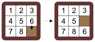
Our goal is to find a sequence of moves from a start state (typically in which the numbers are scrambled) to a goal state, which is typically a state in which all numbers are in order and the empty square is in the lower right, as in the picture above.
We will solve this puzzle in Haskell using a breadth-first search through the state space. We will represent a puzzle state as a list of lists of integers, with 0 representing the empty square:
type Puzzle = [[Int]]
For example, the start state above will be represented as
[ [1, 2, 3], [4, 5, 6], [7, 8, 0] ]
Let's write a function to convert a Puzzle to a nice string representation:
show_puzzle :: Puzzle -> String
show_puzzle p =
    let show_row row = unwords (map show row)
    in unlines (map show_row p)
For example:
> putStr (show_puzzle [ [1, 2, 3], [4, 5, 6], [7, 8, 0] ])
1 2 3
4 5 6
7 8 0
Next we must write a function
neighbors :: Puzzle -> [Puzzle]
that takes any state and returns a list of its adjacent, i.e. neighboring, states. Notice that a state may have as few as 2 or as many as 4 neighbors.
Writing the neighbors
function is a bit tricky. Your first instinct may be to search
for the (x, y) position of the blank square, then to
find all neighboring positions such as (x – 1, y) or (x, y + 1)
that are within the puzzle bounds, and to write a function that can
swap the values in these positions. That could be possible, but it
will be awkward in Haskell. You will probably need to use the !!
operator in various places; using this operator is often a sign that
you are taking an inelegant approach.
In both Haskell and Prolog, it is usually better
if you can find a solution that instead manipulates the data
structure recursively, without using integer indices.
Here is how we can do that in Haskell. First, we will write a
function swap_row that takes a row of
numbers and returns a list of all possible outcomes (if any) of
swapping a 0 with an adjacent number in the row.
> swap_row [1, 2, 0]
[[1,0,2]]
> swap_row [1, 0, 2]
[[0,1,2],[1,2,0]]
> swap_row [1, 2, 3]
[]
It looks like this:
swap_row :: [Int] -> [[Int]]
swap_row (x : y : rest) =
    [y : x : rest | x == 0 || y == 0] ++  -- swap first two elements
    map (x:) (swap_row (y : rest))        -- swap other elements
swap_row _ = []
Notice the use of the partially applied
operator (x:),
which is a function that will prepend x to a given list. This is a
useful trick.
Next, we write a function swap_any_row
that takes a puzzle and returns a list of all possible outcomes from
swapping a 0 with a horizontally adajcent number in any row in
the puzzle:
swap_any_row :: Puzzle -> [Puzzle]
swap_any_row [] = []
swap_any_row (r : rest) =
    map (:rest) (swap_row r) ++      -- swap in first row
    map (r:) (swap_any_row rest)     -- swap in another row
Notice that in both swap_row
and swap_any_row
we are essentially representing a non-deterministic outcome by a list
of possible outcomes. Again notice the use of the partially applied
(:) operator.
Finally, we may find all neighbors of a puzzle state either by swapping horizontally, or by swapping vertically via a transposition operation:
neighbors :: Puzzle -> [Puzzle]
neighbors p =
    let pt = transpose p in
    swap_any_row p ++                      -- horizontal swap
        map transpose (swap_any_row pt)    -- vertical swap
Observe that all of the functions above will work for any board size, not just 3 x 3.
We are now in a position to write a breadth-first search for the goal state. When we find it, we want to return a list of all states from the start to the goal. To achieve this, each element in our breadth-first queue will be a list of states. The head of this list will be a state p which is a state on the search frontier, i.e. a state that is present in the queue. The remainder of the list will be a list of states in reverse order from p back the start state. Our visited set will be a set of states, without a path attached to each state. For now, we will represent both the queue and the visited set using lists.
Our
search function below is somewhat similar to the bfs
graph
search function that we saw above. It takes a start state and a goal
state, and returns a path from the start to the goal if it can find
one, otherwise Nothing.
Here is the implementation:
solve :: Puzzle -> Puzzle -> Maybe [Puzzle]
solve start goal =
  let visit [] visited = Nothing        -- queue is empty, no solution found
      visit (path : queue) visited =
       let p = head path in
           if p == goal then Just path  -- found goal, return path to it
           else let next = (neighbors p) \\ visited   -- unvisited neighbors
                in visit (queue ++ map (: path) next) (next ++ visited)
  in fmap reverse (visit [[start]] [start])
Notice our use of fmap to map a function
over the
contents of a Maybe. This
works because Maybe is a member of the
Functor type class.
Let's choose
a start state in which numbers appear in reverse order,
and try to use our solve function to
find a solution. We'll print out the solution nicely at the end:
test_solve =
    let p = [[8, 7, 6], [5, 4, 3], [2, 1, 0]]
        q = [[1, 2, 3], [4, 5, 6], [7, 8, 0]]
    in case solve p q of
        Just steps -> mapM_ (putStrLn . show_puzzle) steps
        Nothing -> putStrLn "no solution"
Let's run it:
> test_solve
After we wait for 60 seconds, the function is still running. That's not good. What is wrong?
This
is a "real" search problem with tens of thousands of
states. Unfortunately our naive representations of the queue and
visited set as lists are not adequate for a problem of this size. In
particular, the first ++ operation above that appends to the queue,
will run in O(N), and the list
difference operation \\ will also take
O(N).
So we must use more efficient data structures.
Fortunately many structures are available in Haskell's standard
library, though we have not explored them much in this course. To
improve our search's efficiency, let's use a Data.Sequence
to represent the queue. A Data.Sequence represents an arbitrary
sequence of values. It uses a tree-like structure internally and
provides a variety of efficient operations: in particular, we can
prepend or append operations to a Data.Sequence in O(1), and can
concatenate
two sequences in O(log N). We will use a Data.Set
to
represent the visited set. A Data.Set lets us add elements in O(log
N), and also test for membership in O(log N). Internally it uses a
balanced binary tree.
Here is our updated implementation:
import qualified Data.Sequence as Seq
import qualified Data.Set as Set
…
solve :: Puzzle -> Puzzle -> Maybe [Puzzle]
solve start goal =
  let visit :: Seq.Seq [Puzzle] -> Set.Set Puzzle -> Maybe [Puzzle]
      visit queue visited =
        if Seq.null queue then Nothing    -- queue is empty, no solution found
        else let (path, queue1) = (Seq.index queue 0, Seq.drop 1 queue)
                 p = head path in
             if p == goal then Just path  -- found goal, return path to it
             else let next = (Set.\\) (Set.fromList (neighbors p)) visited
                      nextPaths = (map (: path) (Set.toList next))
                  in visit ((Seq.><) queue1 (Seq.fromList nextPaths))
                           (Set.union next visited)  -- add new neighbors to visited set
  in fmap reverse (visit (Seq.fromList [[start]]) (Set.fromList [start]))
Note
that the obscure-looking operator (Seq.><)
concatenates
two sequences.
Our
code is now a bit harder to read, because use fromList
and
toList
in
various places to convert lists to and from sequences and lists. That
is the price we pay for using library data structures rather than
lists. Still, hopefully the code is still readable enough, for a
Haskell function anyway. :)
Let's see if this version is faster:
> test_solve
8 7 6
5 4 3
2 1 0

8 7 6
5 4 0
2 1 3

…

1 2 3
4 5 6
7 0 8

1 2 3
4 5 6
7 8 0

(5.85 secs, 3,105,742,544 bytes)
We have found the solution in about 6 seconds. The 8-puzzle actually
has about 180,000 reachable states (and actually
this search has explored most of them). So it seems that our solution
is reasonably fast, although once again it probably cannot hope to
compete with a solution in a language such as C++ or C#. However, we
could certainly optimize it more. For example, in our solution we
call the transpose
function
often while generating neighboring states, which is relatively
expensive.